cm3060 Topic 05: Text Categorization
Main Info
Title: Text Categorization and Sentiment Analysis
Teachers: Tony Russell-Rose
Semester Taken: October 2021
Parent Module: cm3060 Natural Language Processing
Description
This week we explore the theory underpinning generative approaches to text categorisation and experiment with applying this to real world data.
Key Reading
Jurafsky Martin Chapter 04: Naive Bayes and Sentiment Classification
Jurafsky Martin Chapter 20: Lexicons for Sentiment, Affect, and Connotation
Other Reading
VanderPlas: Chapter 05: Machine Learning (section on multinomial naive bayes)
Lewis et al: The Reuters Corpus (article on development of the Reuters corpus for categorization)
There is a ‘recipe’ from the Antic cookbook also listed among reading, but the book seems not great so skippable.
Lecture Summaries
Week Nine: Text Classification
Intro to text categorization
Introduces spam classification. Then introduces the history of work on the problem of categorization. Starts with 1963 work on Bayesian resolution of Federalist Paper authorship, then topical literature classification.
Formalizes the problem:
We have a fixed set of classes \(C = \{c_1,c_2,\dots ,c_n\}\). A set of labelled documents \((d_1,c_1),\dots ,(d_m,c_m)\). And a document d we want to classify. We need a classifier \(\gamma : d \rightarrow c\).
How do we do this? We could try using rules, but these are difficult to scale and maintain. So we tend to use machine learning now and that’s what the module will focus on. There’s a variety of techniques: naive bayes, logistic regression, support vector machines, or neural approaches.
Bayes’ Theorem and Classification
Introduces the bias in human reasoning that we ignore prior probabilities and look only at the current evidence. A rational judgement would consider both evidence and prior probability.
This leads us to Bayes’ theorem, where we look at the probability of a hypothesis given the evidence: \(P(H|E) = \frac{P(H)P(E|H)}{P(E)}\)
Introduces the terms:
The Prior, this is \(P(H)\)
The Likelihood, this is \(P(E|H)\)
The Posterior, this is \(P(H|E)\)
The Marginal likelihood or model evidence, this is \(P(E)\)
Evidence should be used to update beliefs, not determine them.
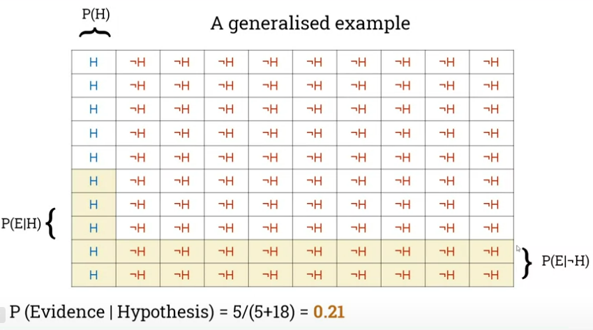
Presents an example with librarians and farmers, then generalizes:

Then turns in the next lecture to Naive Bayes as a baseline classifier.
NB the examples in the lectures are lifted directly from VanderPlas: Python Data Science Handbook, chapter 5.
Very useful as a baseline as it’s fast, with few tunable parameters, suitable to high-dimensional datasets.
How do we adapt the theorem for classification, we can think in terms of features and labels:
\[P(L|features) = \frac{P(L)P(features|L)}{P(features)}\]
To choose between labels we can compare their posterior probabilities:
\[\frac{P(L_1|features)}{P(L_2|features)} = \frac{P(L_1)P(features|L_1)}{P(L_2)P(features|L_2)}\]
So we need to calculate \(P(features|L_i)\) for each label. We can assume a generative model for each label -> features. We specify this model as part of training the Bayesian classifier.
We apply some ‘naive’ assumptions: independence and equality of features’ contributions.
Demonstrates an example of a NB classifier with scikit learn (not text related).
Multinomial Naive Bayes
Here features are generated from a multinomial distribution, so we’re looking at the probability of observing counts across various categories. Find a best-fit multinomial distribution.
Looks at tfidf vectorizer as a way of generating numerical representations of documents and walks through a scikit learn workflow on an existing dataset. The example is taken from VanderPlas: Chapter 05: Machine Learning.
Week Ten: Sentiment Analysis
Introduction to Sentiment Analysis
Gives some examples of sentiment in book reviews (of his own book!).
Introduces some contexts for sentiment analysis. Customer voice and product reviews, public opinion, market prediction.
Introduces the Scherer taxonomy of affective states:
Personality traits: stable personality dispositions and typical behaviour (persist over long term). EG nervous, reckless, jealous, morose
Mood: diffuse non-caused low-intensity long-duration change in subjective feeling. eg cheerful, gloomy, listless, irritable.
Emotion: brief, organically synchronized, evaluation of a major event. Angry, sad, joyful, ashamed, proud, elated, afraid
Interpersonal stances: affective stance towards another person in a specific interaction: friendly, flirtatious, distant, cold, warm, contemptuous
Attitudes: enduring, affectively coloured beliefs, dispositions towards objects or persons, liking, loving, hating, desiring.
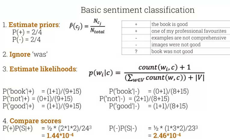
Simplest form of sentiment classification is just positive/negative. With NB we estimate priors, we ignore unknown words, then estimate likelihoods, and compare scores for each class.
Shows an example of classifying a new review with LaPlace smoothing.

For sentiment, occurrence matters more than frequency. We tend to limit counts to binary presence/absence and not bother with TF-IDF or similar.
Negation is obviously really important. A simple baseline is to add a pseudo token NOT_ to any token after the negation before punctuation.
Finally introduces sentiment lexicons. Useful when training data is limited. Some examples:
MPQA Subjectivity Lexicon, 6885 words from 8221 lemmas, 2718 +ve, 4912 -ve.
General Inquirer, similar, more nuanced, sentiment is strong/weak, passive/active, overstated/understated.
One way to use these is to add a feature in classification for whether a word is a member of one of the +ve/-ve lexicons. Could keep running count of these.
Sentiment Analysis using Supervised Learning and Lexicons
The next two lectures walk through some sentiment analysis using nltk. NLTK comes with some classifiers built in, including a NB classifier and DT classifier. Lecture sets up a boolean vector for each document based on inclusion of terms, then trains a couple of classifier models.
This is how he does feature extraction from the tokenized doc:
def document_features(document):
    document_words = set(document)
    features = {}
    #word_features is a corpus list of top N word tokens
    for word in word_features:
	  features['contains({})'.format(word)] = (word in document_words)
    return features
For the lexicon lecture, it features the textblob library, which wraps NLTK and the pattern library to provide a simple API for text processing (see the docs).
,#+BEGIN_SRC python results: silent exports: code from textblob import Textblob
  def get\_blob\_sentiment(sentence):
sentiment = TextBlob(sentence).sentiment
return sentiment.polarity
#+END_SRC
Then shows the approach with NLTK:
import nltk
from nltk.sentiment.vader import SentimentIntensityAnalyzer
nltk.download('vader_lexicon')

def get_nltk_sentiment(sentence):
  sid = SentimentIntensityAnalyzer()
  ss = sid.polarity_scores(sentence)
  return ss['compound']
Lab Summaries
Week Nine lab walks through the multinomial classificaiton problem with no real coding, just playing with the existing code and trying different categories.
Week Ten lab has you try to improve the performance of a sentiment classifier by feature engineering.