cm3015 Topic 02: Classification
Main Info
Title: Classification
Teachers: Jamie Ward
Semester Taken: October 2021
Parent Module: cm3015 Machine Learning and Neural Networks
Description
In this topic we explore supervised learning in more detail, with a particular focus on classification. We introduce two simple, commonly used classifiers: K-nearest neighbours and decision trees. We show how classifiers are typically evaluated using confusion matrices and summary metrics like accuracy, precision and recall.
Week Three: K-Nearest Neighbour and Decision Tree algorithms
Week Four: Classifier Evaluation, Reading, and Labs
Assigned Reading
Alpaydin: Chapter 02: Supervised Learning (section on classification)
Chollet: Chapter O1: What is Deep Learning? (some discussion of decision trees)
Supplementary Reading
Lecture Summaries
2.101: Introduces classification as “a type of supervised learning where the labels on data are discrete or categorical.
2.201: K-Nearest Neighbours
Introduces K-Nearest Neighbours as a simple but effective algorithm for classification. We can measure the distance from our test data object to the objects in our training set. We can find the closest object and assign the same label (if \(k=1\)).
Perhaps that distance is Euclidean, where the distance from \((x_1,y_1)\) to \((x_2, y_2)\) is measured as:
\[\sqrt{(x_2-x_1)^2 + (y_2 - y_1)^2}\]
Or perhaps the distance is Manhattan, where the distance is measured as:
\[|x_2 - x_1| + |y_2 - y_1|\]
If \(k>1\) then we look at the k nearest neighbours. If the neighbours have the same label then we’re OK, otherwise we have a confusion problem.
So K-Nearest neighbours has two input parameters, k, the number of neighbours to look at, and the distance measure to use.
It is a lazy learning algorithm, since we don’t generalize on the training set until we query it.
2.301: Decision Trees
Introduces decision trees as among the most versatile ML algorithms, used for classification and regression, and on complex, non-linear datasets. Particularly useful in random forests.
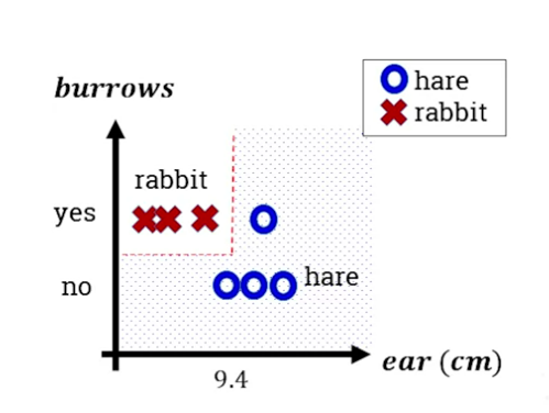
Uses an example of classifying rabbits from hares. Plots a tree with the root node being the most informative question (whether the animal burrows). Interior nodes are subsequent questions used to further distinguish (eg ear length). Leaf nodes are the final labels applied.
Decision trees are white box models, since the tree is explicit so we can see how decisions are made. Shows how we can plot the decision boundaries on a graph:

Decision boundaries can become arbitrarily complex, nonlinear, capturing almost any shape (mentioning that this means it’s subject to the overfitting problem, where it doesn’t generalize well).
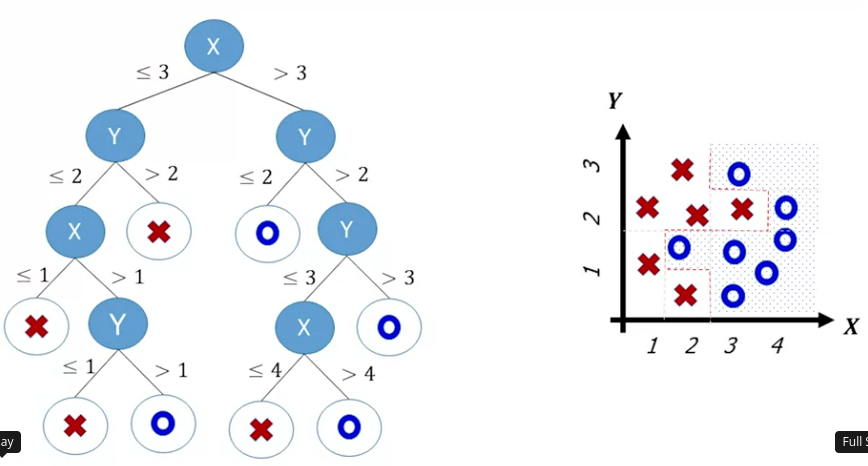
Introduces CART (classification and regresstion tree) as a binary decision tree algorithm. In this algorithm we split the data on a root variable value to minimize the impurity of the resulting groups. Then we recurse down the branches, splitting on more variables. If we find a group that is pure that becomes a leaf node label. For example:

To overcome overfitting we force the model to be simpler, for example restricting the tree depth, or growing it fully and then pruning it.
CART is greedy in training, it works out the optimal split at each stage without considering whether it is overall optimal.
2.501: Classifier Evaluation
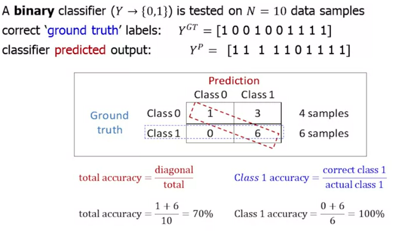
How do we evaluate a classifier? Accuracy is not a great method. Repeats the same material on precision and recall as cm3060 Topic 01: Introduction (see notes on evaluation metrics at the end of that note). Has some additional details on per-class accuracy or class recall:

Lab Summaries
The two labs for this topic implement K-Nearest Neighbours and decision tree classification on the Iris dataset using sci-kit learn. See the note on SKL Nearest Neighbours.