Representing and Mining Text (Provost Fawcett)
Metadata
Title: Representing and Mining Text
Number: 10
Assigned in: cm3060 Topic 02: Basic Processing (section on text representation)
Core Ideas - Working with Text
The chapter presents processing and analysing text data in the context of generating business insights through data science.
Text data presents a challenge to data mining, it is not represented in the feature vector representation that data mining needs. So we need to either engineer the data representation to match the tools, or build new tools to match the data. Generally it’s simpler to try the first approach first, as existing tools are well understood and engineered.
Text is often referred to as ‘unstructured’ data, because it lacks the structure that we expect from data (collections of feature vectors). “Text of course has plenty of structure, but it is linguistic structure - intended for human consumption, not for computers.”
Text is also relatively dirty. Typos, unpredictable acronyms or abbreviations, random punctuation, synonyms and homographs, inconsistent semantics across domains.
Text semantics depends on context - eg “incredible” could be very positive or negative depending on context.
Simple Text Representations (Bag of Words based)
The general strategy in text mining s to use the simplest (least expensive) technique that works.
Some key terms are defined:
- A document is one piece of text, no matter how large or small. A document could be a single sentence or a 100 page report, or anything in between such as a YouTube comment or blog post. Typically all the text of a document is considered together and forms a unit for retrieval or categorization purposes.
A document is composed of individual tokens or terms. Intuitively these are words, though they don’t always map directly to individual words.
A collection of documents is called a corpus.
In text representation, we are taking a set of documents - each a free-form sequence of words - and turning it into a feature-vector of some kind. Each document is one instance, but we don’t know in advance what the features will be. There are several text representations available:
Bag of Words
the [bag of words] approach is to treat every document as just a collection of individual words. This approach ignores grammar, word order, sentence structure, and (usually) punctuation. It treats every word in a document as a potentially important keyword of the document. The representation is straightforward and inexpensive to generate, and tends to work well for many tasks.
If every word is a feature, what is the feature’s value for a given document? In the most basic approach each word is a token and its value is binary, 1 if the token is present, 0 if absent. This approach reduces a document to the set of words contained in it.
Note that the term bag comes from mathematics, where it refers to a multiset, ie a set where members are allowed to appear more than once. The simplest bag of words is really a set of words, with each token appearing once or not at all.
Term Frequency
The next step up in complexity is to use the word count (frequency) in the document instead of just the binary presence or absence. This allows us to differentiate how many times a word is used, useful in some applications where the importance of a term in a document should increase with frequency. This is called the term frequency representation.
Term frequency may be raw counts, or they might be normalized with respect to document length. This helps deal with the issue that some documents might be much longer than others and so their importance could be overstated by raw counts. We might divide the term frequency by the total number of words in the document, for example, to help work around this.
Inverse Document Frequency
Beyond how prevalent a term is in a document, we may care how common it is in the whole corpus. This might help us weight the word’s importance. There are two opposing considerations:
- A term should not be too rare. Say a term occurs once in the whole corpus. Is it important? For retrieval it may be, since a user could be searching for that exact term, but for clustering there is no point keeping a term that occurs once, it will never be significant. So there is often a small, arbitrary lower limit on the number of documents in which a term must occur to be kept in the feature vector.
- A term should not be too common. A term that occurs in every document is not useful for categorization as it doesn’t distinguish anything, or clustering as the entire corpus would cluster together. Overly common terms are usually eliminated through stop words, or an arbitrary upper limit in the number of documents in which a word may occur.
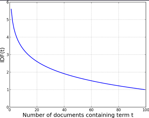
Beyond simple limits, many text processing applications take into account the distribution of the term over a corpus. The fewer documents in which a term occurs, the more significant it likely is to be to the documents that it occurs in. This sparseness of a term t is measured by an equation called inverse document frequency (IDF):
\(IDF(t) = 1 + log(\frac{Total\;number\;of\;documents}{Number\;of\;documents\;containing\;t})\)
Intuitively, IDF is the boost a term gets for being rare. The book shows a graph of \(IDF(t)\) as a function of the number of documents containing t from a corpus of 100. IDF is quite high when the term is rare, reducing quickly to an asymptote of 1.0, most stopwords will have an IDF near one due to their frequency:

Combining TF and IDF
A very popular representation for text is the product of TF and IDF, commonly referred to as TFIDF. The TFIDF value of a term t in a document d is:
\(TFIDF(t,d) = TF(t,d) * IDF(t)\)
The TFIDF score is specific to a single document, while IDF is general over the corpus.
A very common pre-processing workflow is to stem and eliminate stop words from a corpus, before doing term counts. Term counts within the documents form the TF values for each term, the document counts across the corpus form the IDF values. Then each document becomes a feature vector, and the corpus is the set of these feature vectors. This set is then the basis for data mining (classification, clustering, or retrieval).
TFIDF is very common, but not necessarily optimal, often you’d experiment with different bag of words representations for a particular problem to see what works best. Feature selection is often employed to limit the number of terms in the representation, this could be min max thresholds of term counts, and/or using a measure like information gain. (information theory, and information gain is discussed in ch. 3 of the book).
The chapter has a worked example of TF/IDF and an interesting discussion of the relation between IDF and entropy. These aren’t in scope of the module reading so aren’t summarised here.
More Complex Representations - Beyond Bag of Words
Basic bag of words approaches are simple, requiring no parsing ability or linguistic analysis. They perform surprisingly well on a variety of tasks, so are often the first choice for a new problem. But there are applications for which these representations aren’t good enough. More sophisticated representations are available:
N-Gram Sequences
The simplest bag of words treats each individual word as a term, discarding any sequencing information. But in some cases word order is important. A next step up is to include sequences of adjacent words as terms in your representation. This general tactic is called n-grams where n is the maximum number of adjacent words included in a term.
For example if working with bigrams where \(n = 2\), and the text “quick brown fox jumps” we would end up with the tokens:
\({quick,\;brown,\;fox,\;jumps,\;quick\_brown,\;brown\_fox,\;fox\_jumps}\)
If we use “bag of n-grams up to three”, we’d represent each document using as features individual words, bi-grams, and tri-grams.
N-grams are useful when phrases are significant but their component words may not be, eg “exceeded analyst expectations”. They also don’t require linguistic knowledge or complex parsing. But they greatly increase the size of the feature set. So we typically need feature selection or to carefully consider storage.
Named Entity Extraction
Sometimes we need more sophisticated phrase extraction than simple N-grams allow. Something like New York Mets or Game of Thrones in sequence name unique entities with properties and identities that are important. Many text-processing toolkits include a named entity extractor of some kind, often labelling the class of entity extracted.
This process is knowledge intensive though, and need to be trained on a large corpus or hand coded with an extensive database of such names. There are no linguistic principles that can solve the problem with complete accuracy. Often entity extraction is domain specific.
Topic Models
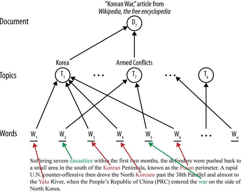
So far the models discussed are created directly from words or entities appearing in the document, and teh resulting model refers directly to words. Sometimes though we want an additional layer between the document and the model. In the context of text this is called the topic layer. It is illustrated by a diagram:

The main idea of a topic layer is first to model the set of topics in a corpus separately. As before, each document constitutes a sequence of words, but instead of the words being used directly by the final classifier, the words map to one or more topics. The topics also are learned from the data (often via unsupervised data mining). The final classifier is defined in terms of these intermediate topics rather than words. One advantage is that in a search engine, for example, a query can use terms that do not exactly match the specific words of a document; if they map to the correct topic(s), the document will still be considered relevant to the search.
Topics are a kind of latent information - an intermediate, unobserved layer of information inserted between the inputs and outputs. Words map to topics (unobserved) and topics map to documents. This makes the model more complex and expensive to learn, but can yield better performance. The latent information is often interesting and useful in its own right.
General methods for creating topic models include matrix factorization methods (eg latent semantic indexing) and probabilistic topic models (eg latent dirichlet allocation). Intuitively, you can think of topic layers as like a clustering of words, learned by the topic modelling process. As with clusters, the topics emerge from statistical regularities in the data. They are not necessarily intelligible or map onto topics familiar to people, though they often do.
The chapter concludes by bringing the techniques together in a case study of mining news stories to predict share prices.