Local Search and Optimization Problems (Russell Norvig)
As discussed in Russell Norvig Chapter 04: Searching Complex Environments
Definitions and Introduction
Local Search algorithms operate by searching from a start state to neighbouring states, without keeping track of the paths, nor the set of states that have been reached. That means they are not systematic - they might never explore a portion of the search space where a solution actually resides. However they have two key advantages: (1) they use very little memory; and (2) they can often find reasonable solutions in large or infinite state spaces for which systematic algorithms are unsuitable. (p. 128)
Local search algorithms can also solve optimization problems, in which the aim is to find the best state according to an objective function.
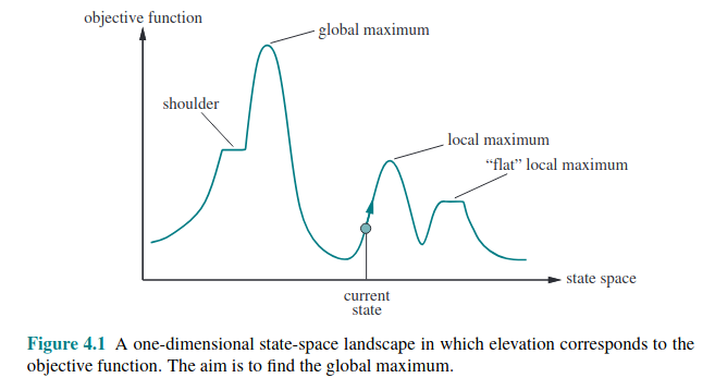
To understand local search we need to understand the state-space landscape as illustrated here:

If the landscape’s elevation is defined by its objective function, the aim is to find the global maximum, and we call the process hill climbing.
If the elevation corresponds to cost, then the aim is to find the lowest valley, or global minimum, and we call the process gradient descent.
Hill Climbing Search
Basic hill-climbing
The hill-climbing search algorithm… keeps track of one current state and on each iteration moves to the neighbouring state with highest value - that is, it heads in the direction that provides the steepest ascent. It terminates when it reaches a “peak” where no neighbour has a higher value. Hill climbing does not look ahead beyond thte immediate neighbors of the current state. (p. 129)
The pseudocode for hill-climbing is as follows:

Hill climbing is called greedy local search because it grabs a good neighbour without thinking ahead. This can perform quite well and make rapid progress. But it can get stuck for any of the following reasons:
Local maxima Hill-climbing algorithms that reach the vicinity of a local maximum will be drawn upward to the peak and then halt.
Ridges result in sequences of local maxima that are difficult to navigate (see p. 131 for an illustration)
Plateaus a flat area of the landscape, could be a flat local maximum or a shoulder from which progress is possible. Hill-climbers can get stuck wandering around plateaus.
In the 8 queens puzzle, steepest ascent climbers get stuck 86% of the time. On the other hand it is quick, taking 4 steps on average when it succeeds, and 3 steps to get stuck (in a state space of 17 million states).
To improve success rate many variations have been made to basic hill climbers. We might allow sideways moves to hope to escape, perhaps with a limit. Stochastic hill climbing chooses at random from uphill moves, basing the probability of selection on the steepness of the ascent. First-choice hill climbing generates successors randomly until one is generated that is better than the current state. Random-restart hill climbing conducts a series of hill climbs from randomly generated start states, it is complete as it will eventually generate a goal state, it will need \(1/p\) restarts where p is the probability of a start state succeeding.
The success of hill-climbing depends on the shape of the landscape. With few plateaus and local maxima it can find a good solution very quickly, but that is not what a lot of landscapes look like. NP-hard problems typically have an exponential number of local maxima to get stuck on.
Simulated annealing
Hill-climbers can get stuck, random walks will eventually find a solution, but will be very inefficient. Could we combine them to do better?
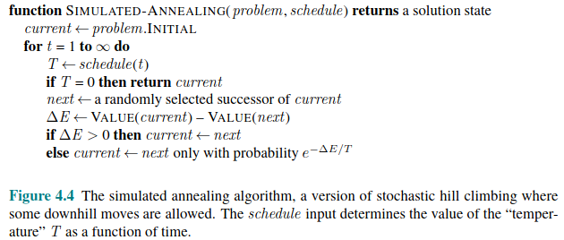
Simulated annealing is such an approach. The metaphor is from metallurgy where annealing is heating a metal to a high temperature then gradually cooling it, hardening it in the process. RN then mix the metaphor by introducing the idea of getting a ball to fall to the lowest minimum in a gradient descent by shaking it out of a local minimum. We have to shake it just the right amount.
Simulated-annealing is similar to hill climbing, but instead of picking the best move it picks a random move, if the move improves the situation it is always picked, but if it doesn’t it will be picked with a probability less than 1. That probability decreases exponentially with the “badness” of the move. The probability also decreases as the “temperature” goes down. The algorithm is shown in pseudocode:

Local Beam Search
In local beam search, instead of just tracking a single state, we start by generating k start states, generate all their successors, and keep the k best successors before repeating.
Is this not just running k random restarts in parallel? No, because “In a local beam search, useful information is passed among the parallel search threads”, rather than each search being independent. The states that generate the best successors have a gravitational pull, so the algorithm abandons unsuccessful searches.
The downside is that they can cluster around small regions of the state space. A variant called stochastic beam search helps with this. Instead of choosing the top k successors, it chooses successors with probability proportional to the successor’s value, increasing diversity.
Evolutionary Algorithms
One class of variants of stochastic beam search are explicitly motivated by the metaphor of natural selection in biology. These are Evolutionary Algorithms. As these are the focus of the first case study in the module, they are broken out to a separate note.