Classification (Alpaydin)
As introduced in Alpaydin: Chapter 02: Supervised Learning
Introduction to Classification
Alpaydin introduces classification through an example where we want to be able to learn the class, C, of “family car”.
We start with a sample of cars, and survey a group of people asking them to label the samples. Those labelled as family cars are positive examples, the rest are negative examples.
Class learning is finding a description that is shared by all the positive examples and none of the negative examples.
If we have learned the class we can either predict whether a new car we haven’t seen before is a family car or not. We can also do knowledge extraction, understanding what properties people associate with family cars.
If after discussion we decide that what sets family cars apart are the price and engine power we can use these two attributes as the inputs to the recognizer. Using this input representation ignores other attributes, like seating capacity or colour.
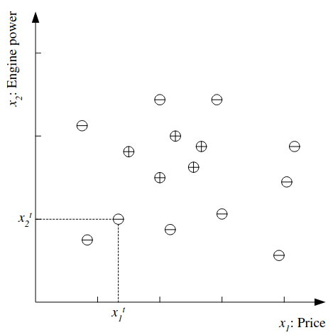
We can denote price as \(x_1\), and engine volume as \(x_2\) with real number representations (in dollars and volume in cubic cm for example). Then each car is represented by a vector of two numeric values \(\mathbf{x} = [ x_1, x_2 ]\).
The label denotes its type:
\[r = \begin{cases} 1\;if\;\mathbf{x}\;is\;positive \\ 0 \;if\;\mathbf{x}\;is\;negative \end{cases} \]
So each car becomes an ordered pair \((\mathbf{x},r)\) and the training set as a whole is:
\[\chi = \{\mathbf{x}^t, r^t\}^N_{t=1}\]
Where t indexes examples in the set. The dataset can be plotted as follows:

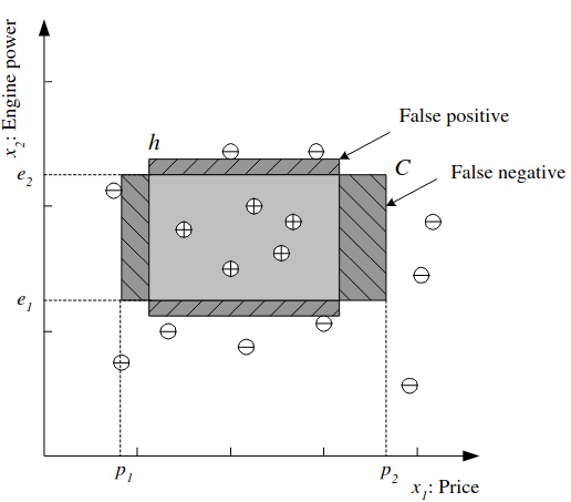
Looking at the data we might identify a Hypothesis class from which we believe C is drawn, for example that the price and engine power are in a certain range: \(\mathcal{H} = (p_1 \leq price \leq p_2) \land (e_1 \leq engine\;power \leq e_2)\).
It is the job of the learning algorithm, then to find the particular hypothesis \(h \in \mathcal{H}\) specified by the quadruple \((p_1^h, p_2^h, e_1^h, e_2^h)\) to approximate C. In other words, to find the values of the parameters. For any hypothesis we can say that \(h(\mathbf{x})\) is 1 if h classifies x as a positive example, or 0 if a negative example.
The empirical error is the proportion of the training data where predictions of h do not match the required values given in \(\chi\):
\[E(h|\chi) = \sum^N_{t=1}1(h(\mathbf{x{^t) \neq r^t)\]
We can visualize this:

We want to find the best hypothesis that meets the challenge of generalization, how well we will classify new examples not part of the training set. If the inputs are real numbered there could be infinitely many hypotheses. We can define the most specific hypothesis, S as that which most tightly covers all the positive examples and no negative ones and most general hypothesis, G as the largest one. Any h between these is a valid hypothesis that is consistent with the training set, and the set of such h is the version space.
A new instance between S and G may be a case of doubt and if errors are costly we may have our system refuse to classify and bump the decision to a human.
A hypothesis class \(\mathcal{H}\) has a capacity, a maximum number of points it can shatter (learn a hypothesis from without error). In practice through these can be pessimistic, as data tends to group together in the real world.
How Many Samples?
How many samples do we need? In probably approximately correct learning, given a class C, and examples drawn from some unknown but fixed probability distribution, p(x) we want to find the number of examples N, such that with probability at least \(1 - \delta\), the hypothesis h has error at most \(\epsilon\) for arbitrary \(\delta \leq 1/2\) and \(\epsilon > 0\). So if \(C\Delta h\) is the region of difference between C and h we want:
\[P\{C\Delta h \leq \epsilon \} \geq 1 - \delta\]
To use the rectangle example, if we take the tightest rectangle we want the probability of a positive example falling in any region between S and G to be upper bounded by \(\epsilon / 4\). The probability that a randomly drawn example misses the strip is \(1 - \epsilon / 4\). That all N miss is \((1 - \epsilon / 4)^N\), that it miss any of the four strips is \(4(1 - \epsilon / 4)^N\), we want this to be at most \(\delta\). Given the inequality \((1-x) \leq exp[-x]\), if we choose N and \(\delta\) such that \(4 exp[-\epsilon N/4] \leq \delta\) then we can also say \(4(1 - \epsilon / 4)^N \leq \delta\), which dividing both sides by 4, taking natural log and rearranging gives us:
\[N \geq (4/\epsilon)log(4/\delta)\]
So with that many samples, and the tightest rectangle as h, with confidence probability at least \(1 - \delta\) a point will be misclassified with error probability at most \(\epsilon\).
Noise
Noise is any unwanted anomaly in the data, and may make the class harder to learn. Noise can come in different forms:
There may be imprecision in measuring the input attributes, shifting the data points in the input space.
There may be errors in labelling the data points (sometimes called teacher noise)
There may be additional attributes not taken into account. Perhaps these are unobservable, in which case they are hidden or latent. These are modelled as a random component and included in noise.
We could make our model more complex to try to account for the noise, but often keeping it simple and accepting some degree of error is preferable since:
It is simpler to use and inspect.
It is simpler to train, and has fewer parameters. A simple model has less variance (changes with new input) but more bias (rigidity and risk of failure). We need to try to minimize variance and bias.
It is easier to explain and extract information.
If there is noise in the training data the simpler model may generalize better. This is an application of Occam’s razor.
Learning Multiple Classes
What if we have more than one class? If we have K classes denoted as \(C_i, i = 1,\dots,K\) and each input instance is in exactly one class then the training set is of the form:
\[\chi = \{\mathbf{x}^t, \mathbf{r}^t\}^N_{t=1}\]
where r has K dimensions and:
\[r^t_i = \begin{cases} 1 \; if \; \mathbf{x}^t \in C_i \\ 0 \; if \; \mathbf{x}^t \in C_j, j \neq i \end{cases}\]
We treat this a set of K two-class problems, we have K hypotheses to learn. The total empirical error is a sum over the predictions for all classes for all instances:
\[E(\{h_i\}^K_{i=1}|\chi) = \sum^N_{t=1} \sum^K_{i=1}1(h_i(\mathbf{x}^t) \neq r^t_i)\]
If we expect all classes to have a similar distribution (ie shapes in the input space) the same hypothesis class can be used for all classes, but in complex classification problems and datasets (like medical diagnostics), this is not the case. EG classifying illnesses may need different hypothesis classes.