Jurafsky Martin Chapter 04: Naive Bayes and Sentiment Classification
Metadata
Title: Naive Bayes and Sentiment Classification
Number: 4
Introduction to Classification
Introduces the Naive Bayes algorithm and its application to text categorization, focusing on the categorization task of sentiment analysis.
Starts by outlining a range of classification tasks: Spam detection, language identification, authorship attribution, taxonomic classification. Notes that subject category classification the task that led to the identification of the Naive Bayes algorithm.
Classification can be thought of more broadly too, including tasks like period dismabiguation (sentence segmentation), word tokenization, and even language modelling and part of speech tagging.
The goal of classification is to take a single observation, extract some useful features, and thereby classify the observation into one of a set of discrete classes.
One way of doing this is hand-written rules. There are many aspects of language processing where handwritten rule-based classifiers remain (part of) the state of the art. But most cases now involve supervised machine learning. JM’s definition is as follows:
Formally, the task of supervised classification is to take an input \(x\) and a fixed set of output classes \(Y = y_1, y_2, \dots, y_m\) and return a predicted class \(y \in Y\). For text classificaiton, we’ll sometimes talk about \(c\) (for “class”) instead of \(y\) as our output variable, and \(d\) (for “document”) instead of \(x\) as our input variable. In the supervised situation we have a training set of \(N\) documents that have each been hand-labelled with a class: \((d_1,c_1),\dots ,(d_N,c_N)\). Our goal is to learn a classifier that is capable of mapping from a new document \(d\) to its correct class \(c \in C\). A probabilistic classifier additionally will tell us the probability of the observation being in the class. This full distribution over the classes can be useful information for downstream decisions; avoiding making discrete decisions early on can be useful when combining systems.
Naive Bayes is an example of a generative classifier, which builds a model of how a class could generate some input data. Given an observation they return the class most likely to have generated the observation. This is in contrast to discriminitive classifiers, like logistic regression or decision trees, which learn what features from the input are most useful to discriminate between the different classes.
Discriminative classfiers are more accurate often, and so more commonly used. But generative classifiers still have a role.
Naive Bayes
The chapter then presents an introduction to Naive Bayes including how it is trained. Full pseudocode is given in the linked note.
Sentiment Analysis
The chapter then presents the optimizations to Naive Bayes used in sentiment analysis, including binarization, discussed in the linked note.
It discusses creating new tokens to deal with negation.
For the latter, we prepend the prefix NOT_ to every word after a token of logical negation (eg n’t, not, no, never) until the next punctuation mark. EG:
didn’t like this movie, but I
Becomes:
didn’t NOT_like NOT_this NOT_movie, but I
This can help well, more sophisticated parsing techniques are also available.
Finally we often use sentiment lexicons to overcome issues of shortage of training data. For example the MPQA lexicon has 6885 words, 2718 positive, 4912 negative. We might use these by adding a feature that denotes ‘this word occurs in the positive lexicon’, and incrementing its value whenever we see a word from the lexicon in the doc.
Other Applications of NB
Since NB doesn’t require that we use all words in our input, and can use any other features we like, it is very flexible.
Spam Detection
In the case of spam detection, we often predefine likely sets of words or phrases as features, and combine them with features that are not purely linguistic. Example features from the SpamAssassin tool:
Email subject line is all caps.
Contains phrases of urgency like “urgent reply”
Email subject line contains “online pharmaceutical”
mentions millions of dollars (regex for large sums)
includes the phrase “one hundred percent guaranteed”
HTML has unbalanced head tags
HTML has low ratio of text to image area
Language Identification
For language id, the most effective features aren’t words at all but character n-grams, or even simpler byte n-grams, where we pretend everything is a string of raw bytes.
Language Modelling
If we do just use word features, and we do use every word in the text, then NB can be viewed as a set of class-specific unigram language models, in which the model for each class instantiates a unigram language model. The model assigns a probability to each word \(P(w|c)\) and so it assigns a probability to each sentence by extension:
\[P(s|c) = \prod_{i \in positions} P(w_i | c)\]
Evaluating Models
The chapter then includes a detailed section on evaluating classifiers. It introduces the familiar confusion matrix, precision, and recall metrics.
It then discusses how to combine these metrics into a single metric. This includes the F-measure, defined as:
\[F_{\beta} = \frac{(\beta^2 + 1) PR}{\beta^2P+R}\]
The \(\beta\) parameter weights the importance of recall and precision, depending on the application need. Values of \(\beta > 1\) favour recall, and vice versa. \(\beta = 1\) equally balances them. it comes from the weighted harmonic mean of precision and recall.
The chapter discusses cross-validation, devsets etc covered in other notes.
Statistical Significance
The chapter also discusses the issue of statistical significance, in the context of comparaing different classifiers. How do we know which is better?
First we can compute the effect size, the difference in some evaluation metric between two classifiers over a test set. Let’s say classifier A is 0.04 better than B over a test set. Can we conclude it’s better? No! It could be accidentally better over that one set. This is where the idea of statistical significance comes in.
We test this by formalizing two hypotheses:
\[H_0 : \delta (x) \leq 0\]
\[H_1 : \delta (x) > 0\]
\(H_0\) is called the null hypothesis. We want to know if we can confidently rule it out, ie we can confidently rule out that A is worse or equal to B and conclude A is better.
We do this by creating a random variable X ranging over all test sets. How likely is it, if the null hypothesis is correct, that among these test sets we would encounter the value of \(\delta (x)\) that we saw. This likelihood is formalized as the p-value: the probability, assuming the null hypothesis is true, of seeing the \(\delta(x)\) that we saw or one even greater:
\[P(\delta (X) \geq \delta (x) | H_0 is\;true)\]
A very small p-value means the difference we observed is very unlikely under the null hypothesis, and we can reject the null hypothesis accordingly. What is the threshold? Commonly 0.05 or 0.01. If the p-value is below these thresholds we say that the result is statistically significant and that we can reject the null hypothesis.
How do we calculate the p-values? In NLP we can’t make assumptions about distributions that are common elsewhere. There are two common tests used in NLP: approximate randomization and the bootstrap test. In paired tests we align two sets of observations, which is natural in this case as we have two classifiers to evaluate. And so we use a paired bootstrap test
The Paired Bootstrap Test
Bootstrapping refers to repeatedly drawing large numbers of smaller smaples with replacement (called bootstrap samples) from an original larger sample. Intuitively, we can create many virtual test sets from an observed test set by repeatedly sampling from it. The only assumption is that the sample is representative of the population. The approach can be applied to any metric.
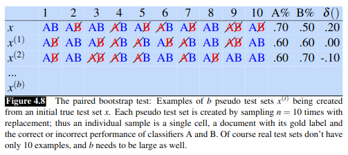
JM walk through an example where we only have 10 documents, and want to test two classifiers, A, and B. We start by recording the results of the two classifiers on the 10 documents, recording the results in row x. Then we create a large number b (say \(10^5\)) virtual test sets \(x^{(i)}\). To create each virtual set we repeatedly select a sell from row x with replacment. Eg to create the first cell of \(x^{(1)}\) we might randomly select the second cell of the x row, then we move on each time randomly choosing (sampling) from the original x. The result looks like this:

Now we have b test sets that provide a sampling distribution, and we can see how often A has an accidental advantage.
One way of doing this is to follow the Berg-Kilpatrick method. Assuming the null hypothesis, we would expect that \(\delta(X)\), estimated over many test sets, would be zero, a much higher value would be surprising. Here, our original test set x happens to be biased by .20 in favour of A, so we compute the p-value by counting over many test sets how often \(\delta (x^{(i)})\) exceeds the expected value of \(\delta{x}\) by \(\delta{x}\) or more:
\[\mathrm{p-value}(x) = \frac{1}{b} \sum^b_{i=1} \mathbb{I}\left(\delta (x^{(i)}) - \delta (x) \geq \delta (x)\right)\]
\[ = \frac{1}{b} \sum^b_{i=1} \mathbb{I}\left(\delta (x^{(i)}) \geq 2\delta (x)\right)\]
Here \(\mathbb{I}(x)\) returns 1 if x is true, otherwise 0 (JM use 1 in the book instead of I, but I can’t typeset that in mathjax).
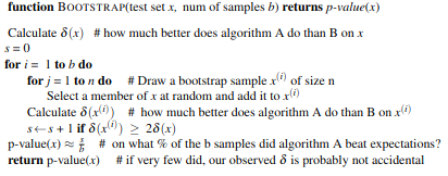
So if we have 10,000 test sets \(x^{(i)}\) and a threshold of 0.01, if we find 47 of the test sets meet the criteria of \(\delta (x^{(i)} \geq 2 \delta (x)\), the resulting p-value of .0047 is smaller than 0.1, indicating \(\delta(x)\) is sufficiently surprising and we can reject the null hypothesis. The full pseudocode is:

Avoiding Harms
The chapter concludes by summarising risks and harms in classification. These include representational harms, caused by a system that demeans a social group. For example a sentiment classifier than assigns more negative emotion and lower sentiment to a racial group systematically.
Another harm might involve censorship. For example toxicity detection has become an important area for detecting harassment, hate speech etc. But such classifiers have been found to, for example, censor posts that just mentioned minority identities. These false positives can lead to the censoring of discourse by and about such groups.
To help identify such issues and make the background of a model explicit we can use a model card, which documents a model with information like:
training algorithms and parameters
training data sources, motivation, and preprocessing
evaluation data sources, motivation, and preprocessing
intended use and users
performance across different demographic or other groups and environmental situations.