Naive Bayes (Jurafsky Martin)
An introduction to training and using a Naive Bayes classifier, as presented in Jurafsky Martin Chapter 04: Naive Bayes and Sentiment Classification
The Naive Bayes Classifier
The ‘naivety’ denotes that the classifier makes a simplifying assumption about how the features in the data interact.
The representation of a document in NB is bag of words (unordered set of words with their position ignored).
NB is a probabilistic classifier, so for a document d, of all classes \(c \in C\), the classifier returns \(\hat{c}\), which has the maximum posterior probability given the document. The hat notation means (our estimate of the correct class):
\[\hat{c} = \mathrm{argmax}_{c \in C} P(c|d)\]
The classifier relies on the familiar rule of Bayesian inference:
\[P(x|y) = \frac{P(y|x)P(x)}{P(y)}\]
Applying the inference rule means we can restate \(\hat{c}\) as:
\[\hat{c} = \mathrm{argmax}_{c \in C} P(c|d) = \mathrm{argmax}_{c \in C} \frac{P(d|c)P( c)}{P(d)}\]
We can drop the denominator \(P(d)\) altogether, since we’ll be estimating every class, and \(P(d)\) doesn’t change for each class, leaving us with \(\mathrm{argmax}_{c \in C} P(d|c) P( c)\).
We can read this as an implicit assumption about how a document is generated: first a class is sampled from \(P( c)\) and then the words are generated by sampling from \(P(d|c)\). Accordingly this is an example of a generative model.
So we generate a classification by taking the product of two probabilities: the prior probability of the class \(P( c)\), and the likelihood of the document \(P(d|c)\). If we represent the document as a set of features \(\{f_1,f_2,\dots ,f_3\}\), that gives us:
\[\hat{c} = \mathrm{argmax}_{c \in C} P(f_1,f_2,\dots ,f_n | c) P( c)\]
This is still too hard to compute, so NB classifiers make two simplifying assumptions. First is the bag of words representation of the features, we assume position doesn’t matter. Second is the naive Bayes assumption, that the probabilities \(P(f_i | c)\) are independent given the class c and so can be ‘naively’ multiplied: \(P(f_1|c) \cdot P(f_2|c) \cdot, \dots, \cdot P(f_n |c)\) to give the overall probability. This gives us the final equation of the naive Bayes classifier:
\[c_{NB} = \mathrm{argmax}_{c \in C} P( c) \prod_{f \in F} P(f|c)\]
This is done in log space to avoid underflow issues, producing a linear combination of the input features (making this a linear classifier). With the words indexed at position i we get:
\[c_{NB} = \mathrm{argmax}_{c \in C} \log{P( c)}+ \sum_{i \in positions} \log{P(w_i|c)}\]
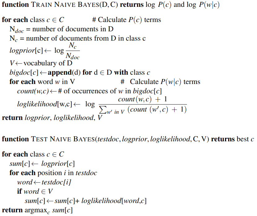
Training the Classifier
How do we learn \(P( c)\) and \(P(f_i | c)\)? One way would be to use the Maximum Likelihood Estimate, and rely on the frequencies in the data.
For \(P( c)\) this is just the number of docs in the class over the number of docs: \(\frac{N_c}{N_{doc}}\).
For \(P(f_i | c)\) we assume the bag of words representation, so we’re looking for \(P(w_i | c)\), which we can compute as the fraction of times the word \(w_i\) appears among all words in all documents of topic c. So we concatenate all documents in c into one large “category c” text. Then we use the frequency of \(w_i\) in that concatenation to give us the likelihood probability. Here V is the union of all word types across all categories:
\[\hat{P}(w_i|c) = \frac{count(w_i, c)}{\sum_{w \in V} count(w, c)}\]
But there’s an issue with this, NB multiplies probabilities, so zeroes cascade. And there will be lots of zeroes.. Here Laplace smoothing (introduced in Smoothing) is used often (unlike in language modelling). This is why we need to take the union of all word counts across all categories.
Generally unknown words in test documents are ignored, we just remove them along (sometimes) with stop words. Generally though stop word removal doesn’t seem to improve accuracy so it’s often skipped.
Pseudocode

Binary Naive Bayes
In some text classification tasks, including sentiment analysis, the presence of the word matters more than its frequency. For these tasks it can improve performance to clip the word counts within each document to 1. This variant is called multinomial naive Bayes or binary Naive Bayes. Note that the counts for each word might higher than 1 within the concatenated document set, if they occur across multiple documents within the cateogry, but are capped at 1 within each doc.