Gradient Descent (Jurafsky Martin)

As discussed in Jurafsky Martin Chapter 05: Logistic Regression.

This is a continuation of the discussion of Learning in Logistic Regression (Jurafsky Martin): Cross-Entropy Loss and Gradient Descent

From here we shall be explicit that the loss function L is paramterized by the weights, which we refer to as \(\theta\) (so in logistic regression, \(\theta = w,b\)). We want to minimize the loss function, averaged over all the examples:

\[\hat\theta = \underset{\theta}{\mathrm{argmin}} \frac{1}{m} \sum^m_{i=1} L_{CE}(f(x^{(i)}; \theta),y^{(i)})\]

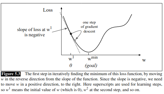
How do we find this minimum? Gradient descent is a method that finds a minimum of a function by figuring out the direction (in the space of the parameters \(\theta\) that the function’s slope is rising most steeply, and moving in the opposite direction. Think of hiking in a canyon and wanting to get to the bottom as quickly as possible. You look all around, see where the ground slopes most steeply and walk down in that direction.

In logistic regression, there is a convenience in that there is just one minimum, with no local minima to get stuck in. As such the loss function is convex. We can visualize this by imagining we randomly initialize the weights with some value \(w^1\). We need the algorithm to tell us whether we should move left or right in the next iteration (make \(w^2\) bigger or smaller) to reach our goal:

The gradient descent algorithm finds the gradient of the loss function and moves in the opposite direction. The gradient of a function of many variables is a vector pointing in the direction of the greatest increase in a function - it’s a multi-variable generalization of the slope.

Once we know the direction, how far do we move? We multiply the gradient by a learning weight \(\eta\). The slope is: \(\frac{d}{dw} L(f(x;w),y)\). A higher learning rate means we move w more each step. This gives us:

\[w^{t+1} = w^t - \eta \frac{d}{dw}L(f(x;w),y)\]

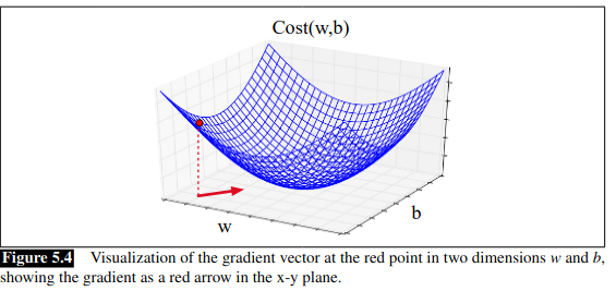
If we imagine two weight dimensions (say an aggregate for w, and one for bias b) the gradient would have two orthogonal components, telling us how much the ground slopes in the w dimension and b dimension:

In actual logistic regression the parameter vector is much longer than 1 or 2 as we have a weight and dimension for every feature. We express the slope in each dimension \(w_i\) as a partial derivative \(\frac{\partial}{\partial w_i}\) of the loss function. The gradient is a vector of these partials:

\begin{equation*} \nabla_\theta L(f(x;\theta ),y) = \begin{bmatrix} \frac{\partial}{\partial w_1} L(f(x;\theta ),y) \\
\frac{\partial}{\partial w_2} L(f(x;\theta ),y) \\
\vdots \\
\frac{\partial}{\partial w_n} L(f(x;\theta ),y) \\
\frac{\partial}{\partial b} L(f(x;\theta ),y) \end{bmatrix} \end{equation*}

And the final equation for updating \(\theta\) based on the gradient is:

\[\theta_{t+1} = \theta_t - \eta \nabla L(f(x;\theta ),y)\]

The derivative of the cross-entropy loss function is:

\[ \frac{\partial L_{CE}(\hat{y},y)}{\partial w_j} = \left[ \sigma (w \cdot x + b) - y \right] x_j\]

The gradient with respect to a single weight w_j is the difference between the true y and our estimated \(\hat{y}\) multiplied by the corresponding input value \(x_j\). The book includes a derivation of this derivative at the end of the chapter.

Stochastic Gradient Descent

Pseudocode

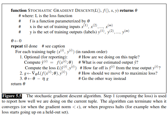
Stochastic gradient descent is an online algorithm that minimizes the loss function by computing its gradient after each training example, nudging \(\theta\) in the right direction. ‘online’ means it processes its input example by examle, rather than waiting to see the entire input. SGD chooses a single random example at a time, moving the weights to improve performance on that single instance.

It includes a hyperparameter, that is a parameter not learned by the algorithm but set by the designer, noted as \(\eta\). \(\eta\) must be adjusted, too high and the learner takes steps that are too large, overshooting the minimum. Too low and the learner will take too long to get to the minimum. Often we start high and then decrease with each iteration, so the learning rate is a function of k, the iteration, and noted as \(\eta_k\).

Section 5.4.3 of the book walks through an example step by step.

Mini-batch Training

The single example-by-example method of SGD can result in very choppy movements, so it’s common to compute the gradient over batches of training instances. In batch training we compute the gradient over the whole dataset. This gives an excellent estimate of which direction to move in, but at the cost of time. A compromise is mini-batch training, where we train on a group of \(1 < m < N\) examples (eg 512, 1024). If \(m=1\) that is Stochastic GD, if \(m=N\) that is batch training.

Mini-batches can be vectorized so the size fits the computational resources available, computing the loss of a mini-batch in parallel. The mini-batch gradient is:

\[\frac{\partial Cost(\hat{y},y)}{\partial w_j} = \frac{1}{m} \sum^m_{i=1} \left[ \sigma(w \cdot x^{(i)} + b) - y^{(i)} \right] x_j^{(i)}\]