Text Classification with Hugging Face
As presented in Tunstall et al: Chapter 02: Text Classification
Presents how to train a classifier, with BERT, following Tokenization with Hugging Face
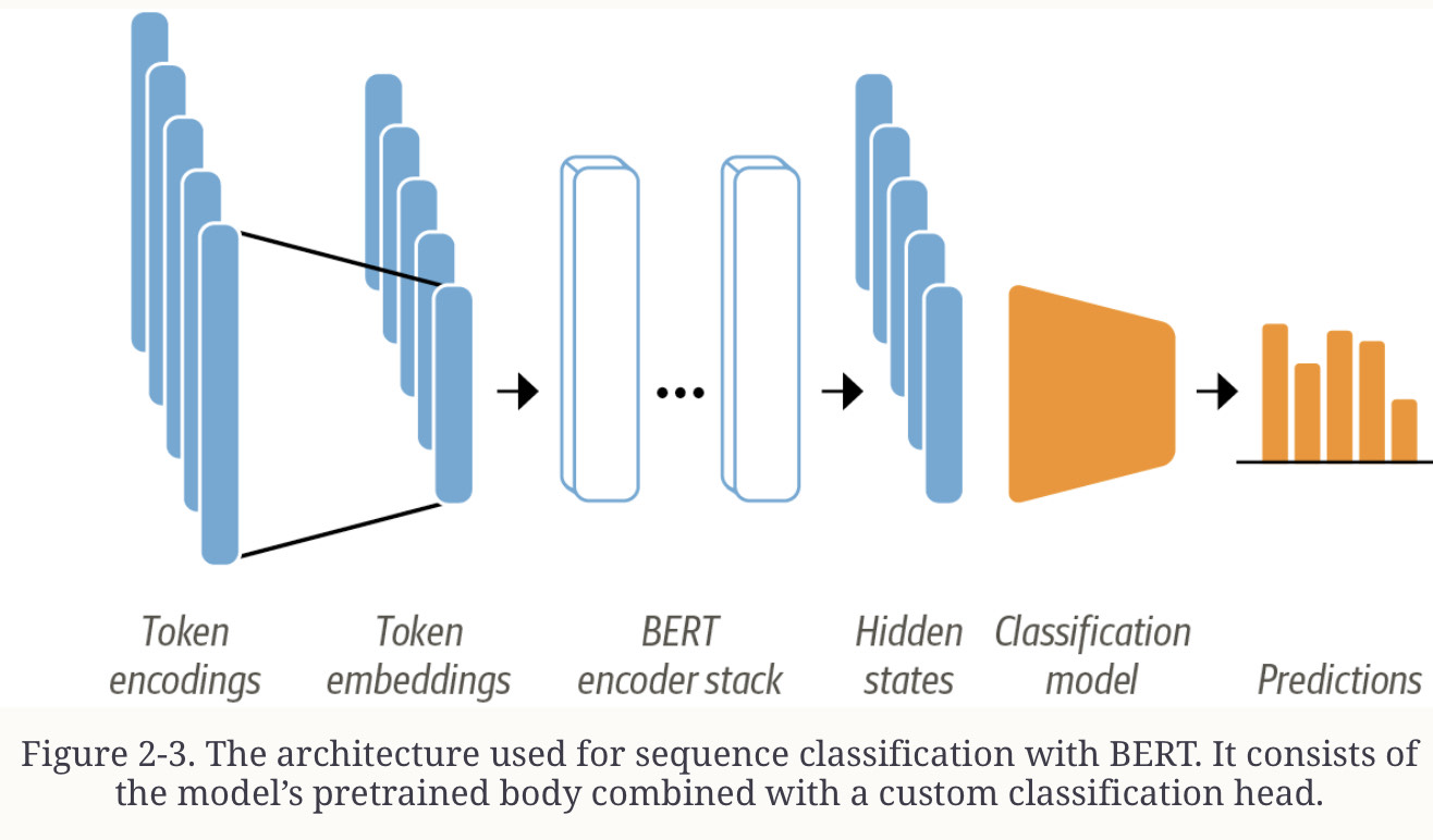
Recall that BERT models are pretrained on masked word prediction. So we can’t use the model directly for classification. We need to modify it. But how? Recall the model architecture:

Text is tokenized and represented as one-hot vectors, whose dimension is the size of the tokenizer vocabulary (50k-100k tokens). Then these tokens are embeddded in lower dimensions and passed through the encoder block layers to yield a hidden state for each input token.
For the objective of masked language modeling, each hidden state is connected to a layer that predicts the token for the input token. For the classification task we have to replace the language modeling layer with a classification layer.
BERT sequences start with a classification token [CLS], so we use the hidden state for the classifiation token as input for our classification layer.
There are two options for training the model on our dataset:
Feature Extraction - we use the hidden states as features and train a classifier on them.
Fine-tuning - we train the whole model end-to-end, updating the parameters of the pretrained BERT model.
Feature Extraction
See the note on Feature Extraction with Transformers (Hugging Face) for the actual process of extracting the features.
Once we have the hidden states we can take a look at them.
Dimensionality Reduction and Visualization
Before we train a model on the hidden states we’ve extracted, it’s a good idea to perform a sanity check.
We use the UMAP algorithm to project the vectors down to 2D. This works best with features scaled to [0,1] so we apply a scaler and use UMAP to do dimensionality reduction:
from umap import UMAP
from sklearn.preprocessing import MinMaxScaler

X_scaled = MinMaxScaler().fit_transform(X_train)

mapper = UMAP(n_components=2, metric="cosine").fit(X_scaled)
df_emb = pd.DataFrame(mapper.embedding_, columns=['X','Y'])
df_emb['label'] = y_train
display_df(df_emb.head(), index=None)

fig, axes = plt.subplots(2,3)
axes = axes.flatten()
cmaps = ["Greys", "Blues", "Oranges", "Reds", "Purples", "Greens"]

for i, (label, cmap) in enumerate(zip(labels, cmaps)):
  df_emb_sub = df_emb.query(f"label == {i}")
  axes[i].hexbin(df_emb_sub["X"], df_emb_sub["Y"], cmap=cmap,
		   gridsize=20, linewidths=(0,))
  axes[i].set_title(label)
  axes[i].set_xticks([]), axes[i].set_yticks([])
Training the Classifier
Once we have the representations and if the sense check suggests that the categories occupy different spaces we can train a simple classifer using, for example, SK-Learn:
from sklearn.linear_model import LogisticRegression
from sklearn.dummy import DummyClassifier
from sklearn.metrics import classification_report

dummy_clf = DummyClassifier(strategy="most_frequent")
dummy_clf.fit(X_train,y_train)
dummy_clf.score(X_valid, y_valid) #0.352

lr_clf = LogisticRegression(n_jobs=-1, penalty="none")
lr_clf.fi(X_train, y_train)
lr_clf.score(X_valid, y_valid) #0.6405

y_preds = lr_clf.predict(X_valid)
plot_confusion_matrix(y_preds, y_valid, labels)

print(classification_report(y_valid, y_preds, target_names=labels)
Fine-Tuning Transformers
If we have the resources required (ie a GPU) and want better results we can fine-tune a Transformer end-to-end instead. See Fine-Tuning a Transformer (Hugging Face).