Jurafsky Martin Chapter 07: Neural Networks and Neural Language Models
Metadata
Title: Neural Networks and Neural Language Models
Number: 7
Core Ideas
Neural networks are a fundamental computational tool in language processing, and have their origins in the 40s and the work of McCulloch-Pitts. But modern uses of neural nets no longer draw on biological inspiration.
In modern neural nets, we have a network of small computing units each of which takes a vector of input values and produces a single output value. This chapter introduces feedforward networks where the computation proceeds iteratively from one layer of units to the next.
Much of the maths behind neural nets is shared from Logistic Regression, but neural nets are more powerful for classification, indeed they can learn any function.
One big difference between logistic regression and neural nets is that in using neural approaches we avoid most uses of rich hand derived features. Instead we build neural networks that take raw words as inputs and learn to induce features themselves as part of the process of learning to classify. Nets that are very deep are particularly good at this, so deep neural networks are particularly good at large scale problems where there is enough data to learn features automatically.
Units
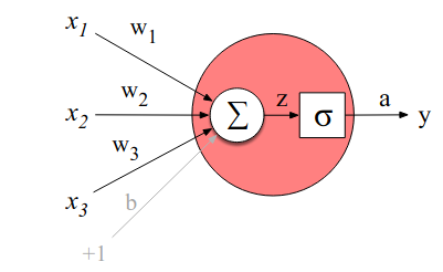
The building block of a neural network is a single computational unit. A unit takes a set of real valued numbers as input, performs some computation on them, and produces an output.
At its heart, this operation is a weighted sum of the inputs plus an additional term, called a bias term. So with a set of inputs \(x_1 \dots x_n\) a unit has a set of corresponding weights \(w_1 \dots w_n\) and a bias b, so the weighted sum z can be represented as:
\[z = b + \sum_iw_ix_i\]
More conveniently, we can use vector notation to describe the operation in terms of the dot product of the weights and input, plus the bias:
\[z = \mathbf{w} \cdot \mathbf{x} + b\]
Neural units don’t just use this value z directly, instead they apply a non-linear function to it, the output of which is called the activation value of the unit, or a: \(a = f(z)\). There are several possible non-linear functions that can be used for f. Three examples are the sigmoid, the tanh, and the rectified lienar ReLU. The sigmoid is presented in detail in Chapter 05: Logistic Regression, to recap it is:
\[\sigma (z) = \frac{1}{1+e^{-z}}\]
and maps the output into the range [0,1]. It’s also differentiable. We can visualize the resulting neural unit:

In practice the sigmoid is rarely used though as an activation function. A similar, and better one is tanh, the output of which ranges from -1 to +1:
\[a = \frac{e^z - e^{-z}}{e^z + e^{-z}}\]
Perhaps the most commonly used though is ReLU which is the same as z when z is positive, otherwise it is 0. Plots of these functions help intuition:

The properties of these functions make them useful for different language applications or network architectures. Tanh is smoothly differentiable and maps outliers toward the mean. ReLU is very close to linear. In the sigmoid or tanh functions, high values of z result in outputs that are saturated, ie close to 1, and have derivatives very close to 0 as a result. Zero derivatives make learning hard, the resulting error signal gets smaller and smaller as you multiply gradients back through a neural network. This is the vanishing gradient problem. ReLU doesn’t have this issue since for high z values its gradient is 1.
There are limits to what a single unit can compute. The chapter walks through an example of logical operations. A single perceptron unit can compute logical and, or, but not xor. A perceptron does not have a non-linear activation function, so is just a linear combination of its inputs. Its output is 0 if the linear combination is \(\leq 0\), otherwise 1. That line acts as a decision boundary, with an output of 0 one side of the line, 1 on the other. xor is a not linearly seperable function.
Neural Networks
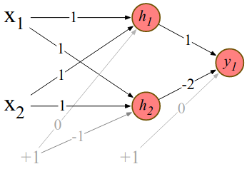
Neural Nets are a solution to this, combining two layers of ReLU units (2 and 1 unit in the layers) we can calculate XOR as follows:

Some points to note on this. After the first layer, the representation of both the inputs \([1,0]\) and \([0,1]\) will be \([1,0]\). This makes it easy to find a linear function to separate them.
Here we specified the weights, but in reality the weights are learned automatically through the backpropagation algorithm. So hidden layers will learn useful representations of their inputs. This is a key advantage.
This solution required a nonlinear activation function (ReLU), a network of linear perceptron units cannot solve it.
A network formed by many layers of purely linear units can always be reduced (ie shown to be compuationally identical to) a single layer of linear units with appropriate weights.
Feedforward Neural Networks
The chapter then introduces the simplest type of neural network, the Feedforward Neural Network in which there are no cycles.
Classification with Feedforward Networks
Recall in previous techniques like logistic regression we crafted features from our texts to use as inputs to the classification model. One way of enriching this with Neural Networks would be to simply add a hidden layer before the final classification. This would allow the network to represent non-linear interactions between the features and would give us a more expressive classifier already.
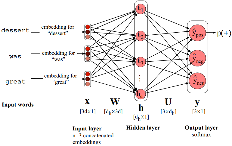
However mostly we do something different. Instead of using our hand-engineered features we draw on deep learning’s ability to learn features from the data by representing words as word2vec or GloVe embeddings. We concatenate the embeddings for the n words in a document and so the classifier becomes:
\[\mathbf{x} = \left[ \mathbf{e}_{w1};\mathbf{e}_{w2};\mathbf{e}_{w3};\dots;\mathbf{e}_{wn}\right]\]
\[\mathbf{h} = g(\mathbf{Wx} + \mathbf{b})\]
\[\mathbf{z} = \mathbf{Uh}\]
\[\mathbf{y} = \mathrm{softmax}(\mathbf{z})\]
Where e is the embedding of the word, and ; denotes concatenation. The output is a probability vector corresponding to our classes.
Relying on another algorithm to have learned useful embedding representations of our words is called pretraining. Using pretrained static or contextual embeddings is a central idea in modern NLP.
