Feedforward Neural Networks (Jurafsky Martin)
As presented in Jurafsky Martin Chapter 07: Neural Networks and Neural Language Models
A feedforward network is a multilayer network in which the units are connected with no cycles. The outputs from units in each layer are passed to units in the next higher layer, and no outputs are passed back to lower layers.
They contrast with, for example, recurrent neural networks where there are cycles. Historically, multilayer networks (esp. feedforward nets) have been called multi-layer perceptrons, but this is a misnomer now as we don’t use perceptrons, we use non-linear activation functions.
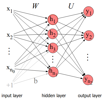
Simple feedforward networks have three node types: input units, hidden units, and output units:

The input layer x is a vector of simple scalar values.
The core of the network is the hidden layer h, consisting of hidden units \(h_i\), each a neural unit. Each layer is fully connected, meaning each unit in each layer takes as input the outputs from all the units in the previous layer, and there is a link between every pair of units from two adjacent layers.
Each hidden unit has a weight vector and bias as parameters. The parameters for the whole layer can be represented in a weight matrix W and a bias vector b. The element \(\mathbf{W}_{ji}\) of the weight matrix represents the weight of the connection from the /i/th input unit \(x_i\) to the /j/th hidden unit \(h_j\).
Now the computaion for the layer is very straightforward. We multiply the weight matrix by the input vector x, add the bias vector b and apply the activation function g (eg ReLU or tanh). Then the output of the hidden layer h is simply:
\[h = g(\mathbf{Wx} + \mathbf{b})\]
Where the activation function applies element wise to a vector. The resulting value h is a representation of the input.
The goal of the output layer is to take this new representation h and compute a final output. The output could be a real-valued number, or a probability. For example, in part of speech tagging we might have one output node for each potential part of speech tag, whose output is the probability of that part-of-speech, and the values of all nodes must sum to 1.
Like the hidden layer, the output layer has a weight matrix (they call it U to distinguish it from W). Some models don’t have a bias vector for the output layer. The weight matrix U is multiplied by its input vector h to return an inermediate result z. z must then be normalized if we are looking for a probability. One function that does this conveniently is softmax as discussed in Jurafsky Martin Chapter 05: Logistic Regression. Recall that this is the same function used in logistic regression. So we can think of a single layer Neural Network as a running standard logistic regression over a hidden representation h, rather than hand-engineered features.
The final equations for a feedforward network then are:
\[\mathbf{h} = g(\mathbf{Wx} + \mathbf{b})\]
\[\mathbf{z} = \mathbf{Uh}\]
\[\mathbf{y} = \mathrm{softmax}(\mathbf{z})\]
This would be a 2 layer network, since we don’t usually count the input layer. Plain logistic regression would be a 1 layer network. See the chapter for notation for deeper networks, and a demonstration of why if all transformations are linear, there is no impact from having more than one layer.
We can also dispense with the bias as a separate vector by just adding an element to our input vector with a value of 1, and then treating the bias as a corresponding weight in the weight matrix. This simplifies the calculations somewhat.