Recurrent Neural Networks
As presented in Chollet: Chapter 10: Deep Learning for Timeseries
A major characteristic of, eg densely connected NNs or convnets is that they have no memory. Each input is processed independently, and no state is preserved between inputs.
To process a sequence with such architectures, you have to show the whole input to the network at once, turning it into a single data point. Such networks are called feedforward networks.
Contrast this to reading text. You process it word by word, section by section, keeping memories of what you’ve read to interpret the meaning of what you are currently reading. We process information incrementally while maintaining some internal model of what we’re processing, built from past information and continually updated as new information arrives.
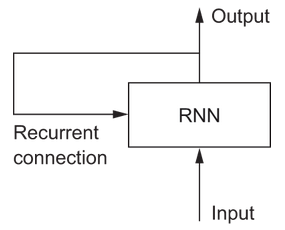
This is the principle adopted by recurrent neural networks, but in a simplified fashion. It processes sequences by iterating through the sequence elements and maintaining a state that contains information relative to what it has seen so far. In effect a RNN is a type of neural network that has an internal loop:

The state of the RNN is reset between processing two different input sequences, so in that sense one sequence is still a single data point. But the data point is no longer processed in one step, instead the network internally loops over the sequence elements.
A Toy Example
Let’s implement a toy forward pass of a RNN to show what’s going on with the state and loop ideas. The RNN will take as input a sequence of vectors of size (timesteps, input_features). It will loop over the timesteps, and at each one consider its current state at t adn the input at t (of shape (input_features,). It will combine them to obtain the output at t. Then that output will become the state at the next timestep.
For the first timestep there is no state, so we set an initial state as an all-zero vector. Essentially:
state_t = 0
for input_t in input_sequence:
    output_t = f(input_t, state_t)
    state_t = output_t

 # or fleshing out /f/
 state_t = 0
 for input_t in input_sequence:
     output_t = activation(dot(W, input_t) + dot(U, state_t) + b)
     state_t = output_t

 # or a detailed NumPy implementation
 import numpy as np
 timesteps = 100
 input_features = 32
 output_features = 64
 inputs = np.random.random((timesteps, input_features))
 state_t = np.zeros((output_features,))

 W = np.random.random((output_features, input_features))
 U = np.random.random((output_features, output_features))
 b = np.random.random((output_features,))
 successive_outputs = []

 for input_t in inputs:
     output_t = np.tanh(np.dot(W, input_t) + np.dot(U, state_t) + b)
     successive_outputs.append(output_t)
     state_t = output_t
 final_output_sequence = np.concatenate(successive_outputs, axis=0)
So a RNN is a for loop that reuses quantities computed during the prior iteration of the loop. That’s it.
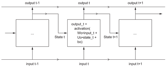
There are a lot of varieties of course. A RNN is characterized by a step function. Here’s another simple example:

Note that the output might be a rank-2 tensor of shape (time_steps, output_features), where each timestep is the output of the loop at time t. A lot of the time you’re only interested in the final output, as it has all the info you want for the whole sequence.
Recurrent Layers in Keras
There are three recurrent layer types in keras, the toy example above corresponds to SimpleRNN. In addition there is LSTM and GRU, which we’ll come onto.
They take inputs of shape (batch_size, timesteps, input_features). Note you can set timesteps to None which enables processing of arbitrary length sequences:
num_features = 14
inputs = Keras.Input(shape=(None, num_features)
outputs = layers.SimpleRNN(16)(inputs)
If you need to process sequences of variable length, this is the way to go. Otherwise fix the size in advance as it enables optimizations and summary stats.
You can run RNN layers in two different modes to either return full sequences of successive outputs for each timestep (a rank-3 tensor of shape (batch_size, timesteps, output_features) or return only the last output for each sequence (ie rank-2 tensor of (batch_size, output_features). You control it with the return_sequences argument to the constructor, False returning only the last output.
Often you want to stack recurrent layers so they learn better representations. In those cases you’ll want the intermediate layers to return the full sequence, and maybe only trim the last layer.
LSTM Layers
Simple RNNs aren’t used in practice much. In practice, long-term dependencies prove impossible to learn due to the vanishing gradient problem, so simple RNNs are stuck learning from very recent experience.
Two other approaches were developed to remedy this, LSTM, and GRU. Long Short-Term Memory or LSTM was developed back in 1997 (see the original paper). GRU is a slightly simpler, streamlined version of LSTM, introduced in 2014 (see the original paper).
LSTM added a way to carry information across many timesteps. Imagine a conveyor belt running in parallel to the sequence you’re processing. At any point, information from the sequence can jump onto the conveyer belt, be carried along, and jump off again when you need it. This is familiar from the residual connections we saw in convnets in Chollet: Chapter O9: Advanced DL for Computer Vision. This is what the LSTM does, saves information for later, to avoid the vanishing gradient problem.
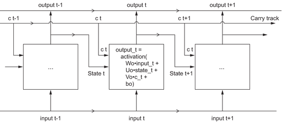
We add to the earlier model of a RNN an additional data flow that carries information across time steps. We call its values at different timesteps c_t where C stands for carry. The carry dataflow is a way to modulate the next output and the next state.
The information it carries is combined with the input connection and the recurrent connection via a dense transformation. IE a dot product with a weight matrix, a bias add, and an activation function. In addition, it affects the state being sent to the next timestep by an activation function and a multiplication operation. Visually:

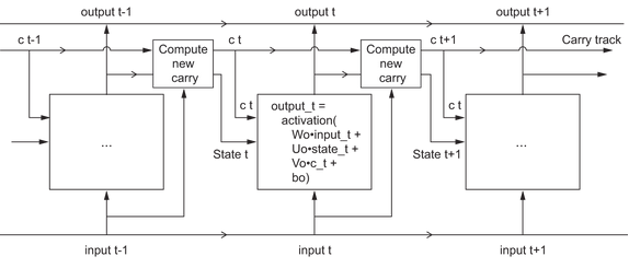
There’s a subtlety - how do you compute the next carry value? This actually involves three distinct transformations. All three have the form of a RNN cell, but all 3 have their own weight matrices. We then combine the three to to get the next carry state.
Putting it all together, you get the full LSTM architecture:

What these operations actually do is determined by the contents of the weights parameterizing them, and those are learned, starting over with each training round. Essentialy they are constraints on the search space, not a design of a solution in the engineering sense.
Probably the search of such constraints is best left to eg genetic algorithms or reinforcement learning. But for now we just need to know that it’s a solution to the vanishing gradient problem and allows information to carry forward longer term.
For more on RNNs, including recurrent dropout, stacking layers, and bidirection, see Chollet: Chapter 10: Deep Learning for Timeseries