Transformer Architecture (Chollet)
As presented in Chollet: Chapter 11: Deep Learning for Text
Introduced in Attention is all you need in 2017, the Transformer architecture quickly overtook RNNs in most NLP tasks.
The idea it introduced, that “neural attention” could produce powerful sequence models without any recurrent or convolution layers became one of the most influential ideas in deep learning.
Self-Attention
As humans read text, they typically skim over some parts, and read other parts attentively, depending on their goals and interests. What if models did the same?
Not all input information seen by a model is equally important, so models should “pay more attention” to some features and less to others.
We’ve already seen variants of this with max pooling in convnets, where the maximum feature value across a region is preserved and the rest discarded. TF-IDF is another version of this idea (a continuous version).
All forms of attention start with computing importance scores for a set of features, with higher scores for more relevant features and lower scores for less relevant ones.
This kind of attention mechanism can be used for more than just highlighting or erasing features. It can be used to make features context-aware. This is really valuable in language. Ideally we wouldn’t have a single static word embedding for a token like “date”, which has several meanings made clearer by the context of the word’s appearance. A better embedding space would provide a different vector representation depending on the words around it.
This is where self-attention comes in. Self-attention modulates the representation of a token by using the representations of related tokens in the sequence. This produces context-aware token reprsentations.
How does it work? There are two main steps to arriving at a new vector representation of a target word in a sentence:
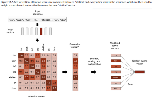
First we compute attention scores, these are relevancy scores between the target word in the input sequence, and every other word in the sequence. A computationally efficient way of doing that is taking the dot product of their vectors.
Second we sum all the word vectors in the sentence, weighted by the relevancy scores. So the target word will contribute a lot to the result, as will closely related words, while irrelevant words will contribute very little. The resulting vector is the new representation of the target word.
We can repeat these steps for every token in the sequence to arrive at a new sequence of vectors. Here’s an illustration of computing the vector for ‘station’ in the sentence: “The train left the station”.

Schematically, the self-attention mechanism is doing the following:
outputs = sum(inputs{C} * pairwise_scores(inputs{A}, inputs{B}))
Note that the inputs are used three times here (given the letters A,B,C). We can translate this as:
For each token in
inputs[A] compute how much the token is related to every token ininputs[B] and use these scores to weight a sum of tokens frominputs[C]
But there’s nothing that requires A, B, C to refer to the same input sequence. In the general case, you could do this with any three sequences.
We call those sequences query, keys, and values. The terminology comes from search engines, and recommender systems. Imagine typing a query “dogs on the beach” to retrieve photos from a database. Each picture in the database has a set of keywords (the keys). The search engine starts by comparing your query to the keys in the database. The values are the photos themselves.
We can restate the operation as:
outputs = sum(values * pairwise_scores(query, keys))
Transformer-style self-attention is operating in this way. You’ve got a reference sequence that describes something you’re looking for: the query. You’ve got a body of knowledge that you’re trying to extract information from: the values. Each value is assigned a key that describes the value in a format that can be compared to a query. You match the query to the keys, and return a weighted sum of values.
In practice, the keys and values are often the same sequence. In translation tasks, for example, the query would be the target sequence, and the source sequence would play the roles of keys and values. For each element of the target (eg “tiempo”) you want to get back to the source sequence (“how’s the weather today?") and identify the bits that are related to it (ie “tiempo” and “weather” should be strongly linked by high attention scores).
If you’re doing sequence classification, the query, keys, and values are the same. You’re just comparing a sequence to itself, enriching each token with context from the sequence.
Multi-Head Attention
That’s not all there is to it though. The original paper was written at a time when the idea of factoring feature spaces into independent subspaces was gaining ground in approaches like depthwise separable convolution.
The paper applies the same approach to attention through the idea of ‘multi-head attention’.
The ‘multi-head’ name refers to the fact that the output space of the self-attention layer gets factored into a set of independent subspaces, learned separately. The initial query, key, and value are sent through three independent sets of dense projections, producing three separate vectors. Each vector is then processed by neural attention, and the three outputs are concatenated back into a single sequence for output.
Each such subspace is called a head. The result looks like this:

The presence of learnable dense projections means the layer can actually learn something, as opposed to being a stateless transformation. Having independent heads allows the layer to learn different groups of features for each token, where features within one group are correlated but are mostly independent from features in another group.
Putting all this together, we can see why the API for MultiHeadAttention looks like this:
num_heads = 4
embed_dim = 256

mha_layer = MultiHeadAttention(num_heads=num_heads, key_dim=embed_dim)
outputs = mha_layer(inputs, inputs, inputs)
The three inputs refer to the query, keys, and values, which happen to be the same often.
The Transformer Encoder
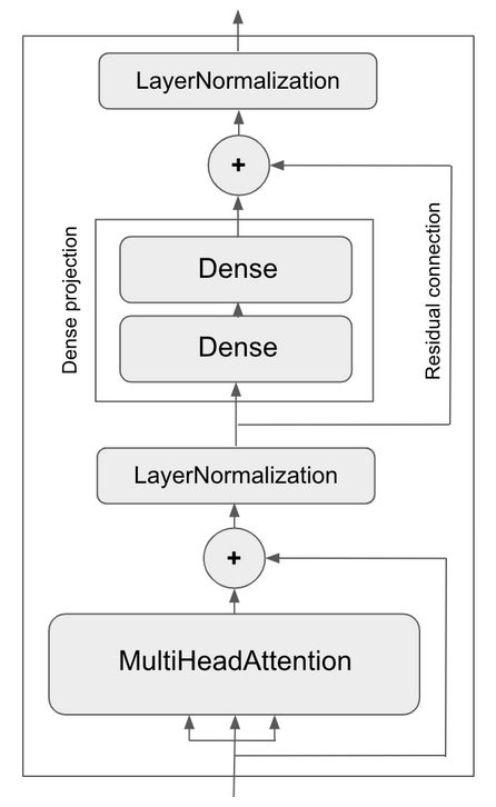
On top of this multi-head attention mechanism, we could add one or two more dense projections to the output. Now it’s deep, so we could add a residual connection to make sure we dont’ lose valuable information. And we can normalize the output too to help backpropagation.
Together, these extra bells an whistles make up the Transformer encoder, one of the two critical parts of the overall Transformer architecture. You can see that they are essentially familiar architecture design patterns of the time, built around the core multi-head attention mechanism.
The architecture of the encoder then looks like this:

A transformer encoder can be used by itself for classification, or in combination with the other critical element, a decoder, for sequence to sequence tasks.
Positional Encoding
There’s still something missing though. By itself, the self-attention model just looks at all the words in its input, as a set. So far we then pass that through dense layers.
Where’s the sequence awareness? We could shuffle the words in a sentence randomly and get the same result from the model we’ve seen so far.
The remedy for this is positional encoding. The idea is simple: we add the word’s position in the sentence to each word embedding. Our input word embeddings will have two components then: the word vector and a position vector which represents the position of the word in the current sentence. The model will have to figure out what to do with that information.
There are different options for positional encoding of course. A naive way would be to just add a ‘position’ axis to the vector and fill it with 0 for the first word in the sequence, 1 for the second and so on. But this would get high values quickly, and we don’t like high values.
In the paper the positional encoding was based on a cosine function and varied cyclically in the range [-1,1]. It’s clever.
Another option is to learn the positional encoding through positional embedding. You learn a positional vector of the same dimensionality as your word index embedding, and then add it to the word index embedding to create a position-aware word embedding.
You need to fix a sequence length in advance in this approach. See p. 345 for an implementation with comments, here it is too:
class PositionalEmbedding(layers.Layer):
  def __init__(self, sequence_length, input_dim, output_dim, **kwargs):
      super().__init__(**kwargs)
      self.token_embeddings = layers.Embedding(
	  input_dim=input_dim, output_dim=output_dim)
      self.position_embeddings = layers.Embedding(
	  input_dim=sequence_length, output_dim=output_dim)
      self.sequence_length = sequence_length
      self.input_dim = input_dim
      self.output_dim = output_dim

  def call(self, inputs):
      length = tf.shape(inputs)[-1]
      positions = tf.range(start=0, limit=length, delta=1)
      embedded_tokens = self.token_embeddings(inputs)
      embedded_positions = self.position_embeddings(positions)
      return embedded_tokens + embedded_positions

  def compute_mask(self, inputs, mask=None):
      return tf.math.not_equal(inputs, 0)

  def get_config(self):
      config = super().get_config()
      config.update({
	  "output_dim": self.output_dim,
	  "sequence_length": self.sequence_length,
	  "input_dim": self.input_dim,
      })
      return config