Jurafsky Manning Lecture Summaries: Topic 18: Ranked Retrieval

18.1: Ranked Retrieval Intro

So far all our queries have been boolean, documents match or not. This is good for experts with precise understanding of the collection and their needs. And it’s good for applications, where IR is embedded in a larger application that can consume 1000s of results easily.

But it’s not good for the majority of users. Most users are incapable or unwilling to write Boolean queries. They certainly don’t want to wade through 1000s of results.

Boolean search often has a feast or famine problem, they return too few (0) results, or too many.

It takes skill to get good results, if you use AND you get too few, OR you get too many.

The solution to this has been ranked retrieval models. Rather than a set of documents satisfying a query expression, in ranked retrieval models the system returns an ordering over the (top) documents in the collection with respect to the query.

Accompanying this has been the adoption of free text queries. Rather than a query language of operators and expressions, the user’s query is just one or more words in a human language.

In principle these are two separate choices, but in practice they have been coupled.

In ranked retrieval, when a system produces a large result set it’s not an issue, we just show the top k (c. 10) results and don’t overwhelm the user.

The premise, is that the ranking algorithm scores well. We wish to return in order the documents most likely to be useful to the searcher.

How can we rank-order the documents in the collection with respect to the query? We assign a score say in [0,1] to each doc. This score measures a match between query and doc.

Let’s start with a single term query. If the query doesn’t occur in the doc, we can score it as 0. Otherwise the more frequent the term occurs, the higher the score should be.

There are different alternatives for this frequency scoring.

18.2: Scoring with the Jaccard Coefficient

The Jaccard coefficient is a commonly used measure to score the overlap of two sets. It is simply:

\[\mathrm{jaccard}(A,B) = \frac{| A \cap B |}{| A \cup B|}\]

A Jaccard coefficient of a set with itself will be 1. If the two sets are disjoint the coefficient will be 0. So we always get a number between 0 and 1 and the sets can be different sizes.

What if we use the jaccard coefficient to score the query-document match. Note that some documents might win because they are shorter (the set union will be smaller). In fact several IR models prefer shorter documents.

There are issues with this approach. It doesn’t consider term frequency. Also rare terms in a collection are more informative than frequent terms.

Also, we need a more sophisticated way of normalizing for length. Later we’ll look at cosine similarity. It turns out the cosine similarity for just a binary bag of words is $\frac{| A \cap B | }{\sqrt{| A \cup B|}}$.

This turns out to be better for normalization.

18.3: Term Frequency Weighting

Term frequency weighting is one of the components regularly used in actual IR systems.

We can start by going all the way back to the term-document incidence matrix from the start of the topic. Each column vector here was a boolean vector representing a document, the length of which was the size of the vocabulary.

Instead of Boolean incidence, we can record the frequency instead. So the matrix has the same dimensionality but the values are Real numbers, instead of booleans.

Now we’ve moved from sets of words, to a bag of words. There are limitations of course, word order is not considered. This is a step back from positional indices. We’ll look later at how to get that positional info back.

For now we focus on the bag of words itself. The term frequency $tf_{t,d}$ is defined as the number of times t occurs in d. How do we make use of this in scoring matches?

We don’t want to just apply the frequency linearly - a doc which mentions my query 30 times is probably not 30x more relevant than a doc that mentions it once.

Standardly now we look at log-frequency weighting where the weight of term t in d is $1 + \log_{10} \mathrm{tf}_{t,d} \; \mathrm{if} \; \mathrm{tf}_{t,d} > 0$, otherwise 0.

This produces less than linear growth.

For a multi-word term, we’ll take the sum of the query-document term pairs. Note that we can just take the intersection of words in query and doc as these are the only words that will affect the score:

\[\mathrm{score} = \sum_{t \in q \cap d} \left( 1 + \log \mathrm{tf}_{t,d} \right)\]

The score is still 0 if none of the terms is present in the doc.

18.4: (Inverse) Document Frequency Weighting

The idea behind using doc frequency is that rare terms are more informative than frequent terms.

Consider a term in a query that is rare in the collection. A doc containing this term is very likely to be relevant to the query. So we want to give a high weight for rare terms.

On the other hand, frequent terms are less informative than rare terms. A doc containing a frequent query term is more likely to be relevant than if it doesn’t contain it, but it’s not such a sure indicator of relevance.

So for frequent terms, we want some positive weight, but lower weights than rare terms. We use document frequency to do this.

$\mathrm{df}_t$ is the document frequency of t: the number of documents that contain t. It is an inverse measure of the informativeness of t. $\mathrm{df}_t \leq N$.

Then we define the inverse document frequency (IDF) of t by:

\[\mathrm{idf}_t = \log_10 \left(\frac{N}{\mathrm{df}_t}\right)\]

We use the log to “dampen” the effect of idf. The base of the log is immaterial. A word that occurs in every document will then have a weight of 0.

Note that idf values don’t change with the query, they will be the same regardless of query.

Note that also idf values have no effect on one term queries, since the same idf scaling score will be applied to every document.

Another frequency measure is collection frequency - the number of occurrences of t in the whole collection, counting multiple occurences in each document.

Why don’t we use this instead of document frequency? It’s the document frequency that captures the aboutness of a document more. Take an example like “try” and “insurance” in the sample corpus they have similar collection frequency, but insurance has much lower document frequency. This suggests that “insurance” is the more relevant term to capture from the query in matching a document. That’s the intuition behind using doc frequency rather than collection frequency.

18.5: TF-IDF Weighting

We now put the TF and IDF together to create the tf-idf weight:

\[w_{t,d} = \left( 1 + \log \mathrm{tf}_{t,d} \right) \times \log_{10} \left(\frac{N}{\mathrm{df}_t}\right)\]

This is the best known weighting scheme in information retrieval.

It increases with the number of occurences within a document. It also increases with the rarity of the term in the collection.

So our final ranking of documents for a query is:

\[\mathrm{Score}(q,c) = \sum_{t\in q\cap d} \mathrm{tf.idf}_{t,d}\]

So we’ve gradually moved from binary vectors, to count vectors, to a weight matrix. Now each document is a real-valued vector of dimensionality $|V|$ where each element in the vector is its real-valued tf-idf weight.

18.6: The Vector Space Model

We saw in the last lecture that we now have a $|V|$-dimensional vector space where the terms are the axes of the space, and documents are points or vectors in the space.

This is very high-dimensional, there would be tens of millions of dimensions in the case of a web-search engine. The vectors would be very sparse, most entries are 0.

The queries are then treated in the same way, they are vectors in the same space.

Then we can rank documents according to their proximity to the query in the space.

Proximity is the similarity of the vectors, or roughly the inverse of the distance.

We do this because we want to get away from the in-or-out boolean model.

How do we calculate the promixity?

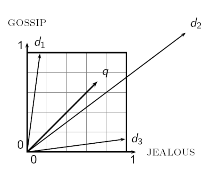
A first stab might be Euclidean distance. But the issue is that the distance is large for vectors of different lengths. Have a look at this example:

Instead of distance, we want to look at the angle between the vectors.

As a thought experiment, imagine concatenating a document to itself. The Euclidean distance would be large, even though semantically they are the same. The angle between them would be 0, which captures this.

For the angle, note that ranking documents in decreasing order of the angle between query and doc is equivalent to ranking them in increasing order of the cosine of the query and doc.

So we will often hear the phrase “cosine similarity”. Why cosine? Well notice that the cosine of an angle of 0 is 1, and of an angle of 180 it is -1. So the cosine is a monotonically decreasing function for the interval [0,180].

So why not reciprocal or negative of the angle? Because there is an efficient way to calculate the cosine using vector algebra.

We start by normalizing the length of the vector by dividing each of its components by its length, using the $L_2$ norm to calculate the length.

This gives us a unit vector touching a unit hypersphere around the origin. So now long and short documents have equal weights.

To take the cosine of a query and doc then, we take the dot product of the two vectors normalized in this way.

18.7: Calculating TF-IDF Cosine Scores in an IR System

There are a lot of variants to TF-IDF measures:

The single letters in this table denote the names of the weighting approach in the SMART notation.

Weighting might be different with queries vs. documents. So SMART notation would look like ddd.qqq for the approaches to document and query.

A very standard scheme is lnc.ltc:

Document: logarithmic tf, no idf, cosine normalization.

Query: logarithmic tf, idf, cosine normalization.

Why no idf on the document? You’ve already factored idf into the query. There are some advantages for efficiency.

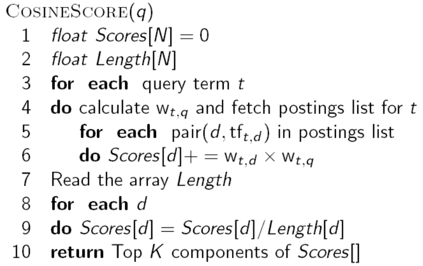
Putting it together here’s a rough algorithm for the top results based on cosine similarity:

We can skip the length normalization of the query as it won’t change the ranking result.

Note that this isn’t yet practical, we might have billions of documents, and we need some efficient way of selecting likely docs and sorting the scores. But it’s the rough idea.

18.8: Evaluating Search Engines

How do we measure a search engine?

We might measure how fast it indexes, (number of docs/hour)

How fast does it search (latency as a function of index size)

Expressiveness of the query language, speed on complex queries, ability to express complex information needs.

Unclutterd UI, price of use.

These are all quantifiable, but the key measure is user happiness.

Blindingly fast, useless answers won’t make a user happy. We need a way of quantifying user happiness based on result relevance.

Relevance is assessed relative to the information need, not the query.

How do we do this? If we have a benchmark document collection, a benchmark set of queries representing info needs, and we gather assessor judgments of whether docs are relevant to queries - then we can use precision/recall/f-measure.

To evaluate ranked results, we need to go further. The system can return any number of results. By taking various numbers of the top returned documents (levels of recall) the evaluator can produce a precision-recall curve.

We can also calculate mean average precision. We calculate the average precision for each recalled match for a query. Then we take the macro average, we average the average over a set of queries.

Alex's Notes