cm3035: SQL Lecture Summaries
From CM3035 Topic 02: Database Schemas and ORMs
2.1 Intro to Relational Datbases
2.102 Intro to Relational Data
The relational model approach is one in which tuples of data points have defined relations to each other.
The atomic unit is the data type, typically strings, integers, dates, booleans etc.
The relation is represented as a table. The columns of the table are attributes, the rows are tuples representing an entity.
The subject matter of the table (People, Accounts) is known as the relvar.
Candidate keys are those which uniquely identify an entity. Foreign keys link entities in different tables.
See CM3010 Topic 02: Relational Databases for more.
2.105 Building a Database
Walks through setting up a database in postgres.
To login to postgres use psql -d <dbname> db name is required, you can use the postgres database, which is an admin database, if you don’t want to jump straight into another one.
Thereafter it’s standard SQL, so CREATE DATABASE <dbname>;
Postgres commands start with a backslash, so \list for example shows the databases.
\c <dbname> is a connection command, like use <dbname>; in MySQL.
Once connected you can use \d like describe in MySQL. \d on its own will list the tables \d <table_name> will show the attributes in the table.
You can issue a shell command from within the postgres repl with \! eg \! clear to clear the terminal.
Postgres enforces single quotes for strings. Creates some tables and inserts some data.
2.106 Relational Modelling Limitations
Binary data is a form of unstructured data that presents a challenge for data modelling in web apps. Postgres provides a BLOB type, a Binary Large OBject, which we can use to store binary data.
Alternatively store the binary data in the file system (or S3 Bucket) and store its address in a VARCHAR field.
Neither option allows us to index or query the content of those files. We could potentially annotate the files with metadata, manually or automated, to give us something to search.
Related is the issue of documents. It’s easier to extract text from a text document, but any complex document is not going to be easily summarised by relational tables.
Plus any large document store is likely only going to be useful with full text search enabled for users.
If you need document storage and search you’re likely going to need more than a relational DB, you can look at Apache Jackrabbit or Apache CouchDB.
Postgres does support JSON data and some limited full text search.
Another modelling change for relational DBs is graph data. Walks through a really weird implementation of a graph in relational terms before showing a more sensible approach of having an edge table.
What about hierarchical data, like a tree? You can model it, but the issue comes down to querying and tree traversal. If we include a ‘parent’ column as representing our edge, traversing the tree becomes a matter of multiple queries to track each parent.
This does not work well with common graph search questions - shortest path, largest subset, subset comparison etc. We need high volumes of queries to answer this in a relational db. Typically we’d then have to take all the data out of the DB, and crunch it in a programming language.
Alternative DBs are built to make such queries efficient, eg neo4j. These can be very useful for web applications that are network driven (like a social network).
When starting a new web app, you should think about what data, files, or info you’re collecting from users, and how you’re going to index, search, and return them to users. Then consider what system provides the most natural representation of the data you’re working with.
2.107 Database Good Practice
Introduces normalisation as a process of disaggregating datasets to avoid duplications.
It helps:
Free the collection of relations from undesirable insertion, update, and deletion dependencies;
Reduce the need for restructuring the collection of relations, as new types of data are introduced, and thus increase the life span of applications;
Make the relational model more informative to users;
Make the collection of relations neutral to query statistics, where those will change
(Codd, Further normalization, 1972)
In practice, we have different levels of normalization defined as normal forms. Each level structures the data such that it more closely adheres to the spec defined by Codd.
As a minimum we should consider a normalized database as being in third normal form or higher.
Each NF is dependent on the previous ones.
First Normal Form
Our data is indexed with a unique primary key, there are no repeatining unit groups, and our data is atomic.
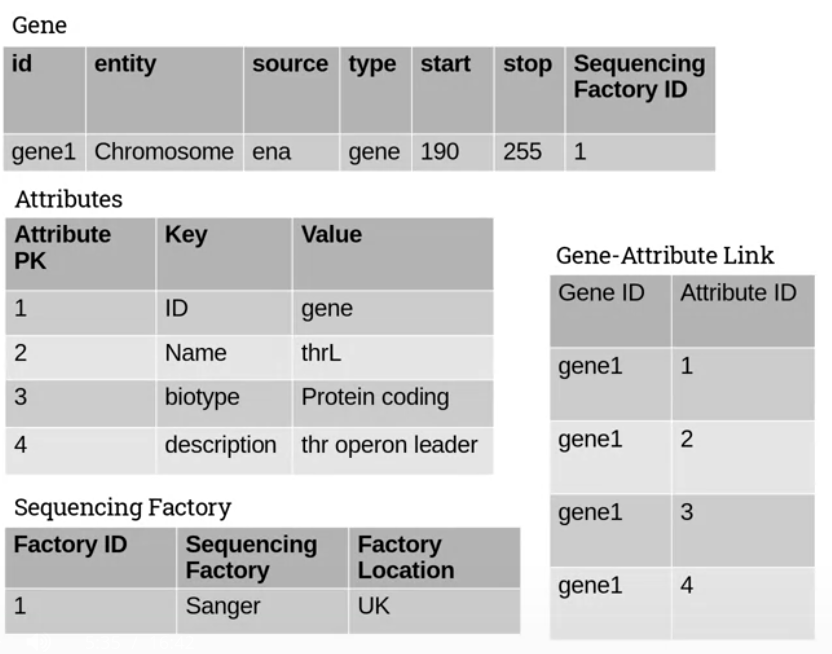
Consider a table which has a column for ‘attributes’ or ‘http headers’ that contains a series of key value pairs. To satifsy first normal form we’d need to disaggregate this column.
One way would be to have a column for each key in the key value pair. But what about when the number of key value pairs is variable/unpredictable? When we encounter a new key we’ll have to change our db schema to add a new column.
Instead we can add a new table for the attributes, with columns for the key and value. Then add a link table which pairs a key-value combo with the original entity. This way our key-value table only has as many rows as there are possible combinations.
We can also check for other entities listed in our source table. Imagine we have a table for genes and it has a column for the sequencing factory. These are different things. So create a table for the factory and link it back to the gene.
Here’s a structure that reflects this approach:
Second Normal Form
Second and Third normal forms relate to primary key dependencies, we want to separate out our data to avoid dependencies.
Take this example:
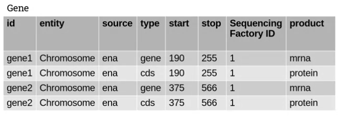
If you look at the product column you’ll see that it’s dependent on the id and type columns. If we know the id and type, we can predict the product with certainty.
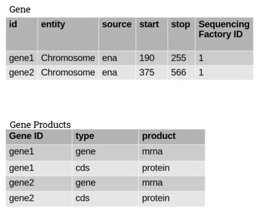
second normal form requires that we remove such dependencies where a column value is dependent on aggregates including the primary key.
We pull out the dependent and independent columns into their own table like this:
Third Normal Form
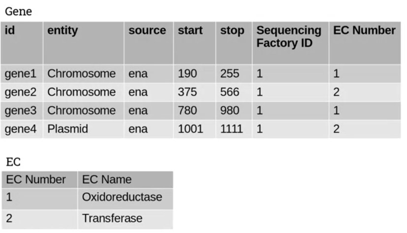
Third normal form requires the removal of transitive dependencies, where the value of one column is dependent on the value of another, non-primary key column.
Consider this example:

The values of EC Number and EC Name seem to depend on one another. One of these columns has redundant data and we can extract it to another table as follows:
2.2 SQL
2.202 walks through queries in the Postgres REPL, inserting genes into the database created in the last section.
Highlights the CURRVAL function in Postgres which returns the latest value in a sequence. Sequences are named separately in Postgres, so you can call CURRVAL('sequence_name') to get the most recent value.
This is really helpful in adding new entities in tables with foreign keys (in single user scenarios I guess), you don’t have to keep and use the linked foreign key if you’ve just added it.
Runs through basic querying, also covered in cm3010: Databases and Advanced Data Techniques.
2.204: Joins
Extends to joins. Joining is essentially the reverse of the normalization process that we went through in designing the db.
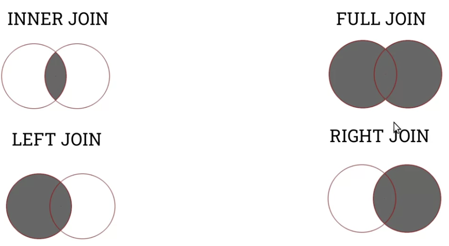
There are four main types of join:
INNER JOIN only returns results where the first and second table satisfy the join requirement (ON).
LEFT JOIN returns all rows from the first table, and only rows from the second that satisfy the join requirement.
RIGHT JOIN is the expected reverse of this.
FULL JOIN returns all rows, regardless of match.
It’s easy to visualize them in terms of set operations:
2.205: Performance
If we’re not careful with query construction performance can be slow, if the db is building the Cartesian product of our tables, then filtering, this will be expensive.
This is an issue in web apps where the user expectation is for action within a short time.
There are a number of things we can try to improve performance.
One of the simplest techniques is a table index. If we’re frequently querying based on one column (SELECT ... FROM ... WHERE column='query'), we create an index for that column.
The index creates a fast lookup table for the column values.
We create a column index like this: CREATE INDEX <index_name> on <table> (<column>);
For joins, introduces the EXPLAIN and EXPLAIN ANALYZE methods of seeing what’s happening under the hood and modifying expensive queries.
If we find an expensive join, we can consider techniques like nesting subqueries. For example filtering a table first on a column index before joining it.
Like this:
SELECT sub.*, ec.*
FROM
  (SELECT *
   FROM
     genes
   WHERE
     entity='Chromosome) sub
  JOIN
    ec
  ON
    sub.ec_pk=ec.pk
Now the join is working with much less data.
If we find our application is frequently joining large tables, there are some other techniques to try.
The first is to actually alter the database design to denormalise a little. This is often not a good idea.
Alternatively we create a materialized view, a kind of adjunct table that contains the contents of a query. We do it like this:
CREATE MATERIALIZED VIEW gene_ec_view
AS
SELECT
  gene_id,
  entity,
  source,
  start,
  stop,
  sequencing_pk,
  ec_name
FROM
  genes,
  ec
WHERE
  genes.ec_pk=ec.pk;
These views in Postgres do not auto-refresh when the underlying data changes, you have to manually refresh them: REFRESH MATERIALIZED VIEW <view_name>;
2.207 SQL Functions
Walks through some aggregate functions. SELECT COUNT(*) FROM <table>; returns a quick count of the number of rows.
Also shows numeric functions: MIN, MAX, SUM, AVG. You can compose functions like ROUND(AVG(<column>))
String functions include UPPER and LOWER to cast the column strings to upper and lower case, also LENGTH which returns the length of the strings in the columns.
For date functions you can do SELECT NOW() to get the current date and time if you want a timestamp column just insert NOW().
Shows a quick GROUP BY example.
2.208 Altering the DB
Walks through the DROP command to completely remove databases or tables.
What if we want to remove a column? We can use the ALTER command: ALTER TABLE <table> DROP COLUMN <column> [CASCADE];
To add a new column: ALTER TABLE <table> ADD COLUMN <column> <TYPE> [DEFAULT(<VALUE>)];
To update values:
UPDATE <table> SET <column>=<value> [WHERE...];